10.9 - Reducing Structural Multicollinearity
Recall that structural multicollinearity is multicollinearity that is a mathematical artifact caused by creating new predictors from other predictors, such as, creating the predictor x2 from the predictor x. Because of this, at the same time that we learn here about reducing structural multicollinearity, we learn more about polynomial regression models.
An Example
What is the impact of exercise on the human immune system? In order to answer this very global and general research question, one has to first quantify what "exercise" means and what "immunity" means. Of course, there are several ways of doing so. For example, we might quantify one's level of exercise by measuring his or her "maximal oxygen uptake." And, we might quantify the quality of one's immune system by measuring the amount of "immunoglobin in his or her blood." In doing so, the general research question is translated into the much more specific research question: "How is the amount of immunoglobin in blood (y) related to maximal oxygen uptake (x)?"
Because some researchers were interested in answering the above research question, they collected the following data (exerimmun.txt) on a sample of 30 individuals:
- yi = amount of immunoglobin in blood (mg) of individual i
- xi = maximal oxygen uptake (ml/kg) of individual i
The scatter plot of the resulting data:
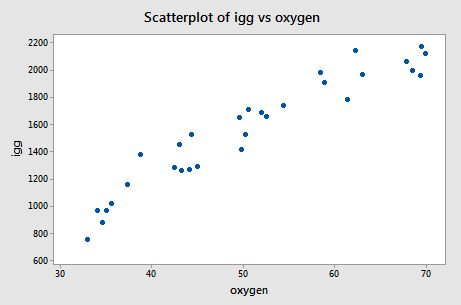
suggests that there might be some curvature to the trend in the data. In order to allow for the apparent curvature —rather than formulating a linear regression function —the researchers formulated the following quadratic polynomial regression function:
\[y_i=\beta_0+\beta_1x_i+\beta_{11}x_{i}^{2}+\epsilon_i\]
where:
- yi = amount of immunoglobin in blood (mg) of individual i
- xi = maximal oxygen uptake (ml/kg) of individual i
As usual, the error terms εi are assumed to be independent, normally distributed and have equal variance σ2.
As the following plot of the estimated quadratic function suggests:
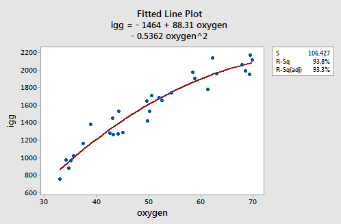
the formulated regression function appears to describe the trend in the data well. The adjusted R2-value is 93.3%.
But, now what do the estimated coefficients tell us? The interpretation of the regression coefficients is mostly geometric in nature. That is, the coefficients tell us a little bit about what the picture looks like:
- If 0 is a possible x value, then b0 is the predicted response when x = 0. Otherwise, the interpretation of b0 is meaningless.
- The estimated coefficient b1 is the estimated slope of the tangent line at x = 0.
- The estimated coefficient b2 indicates the up/down direction of the curve. That is:
- if b2 < 0, then the curve is concave down
- if b2 > 0, then the curve is concave up
So far, we have kept our head a little bit in the sand! If we look at the output we obtain upon regressing the response y = igg on the predictors oxygen and oxygen2:
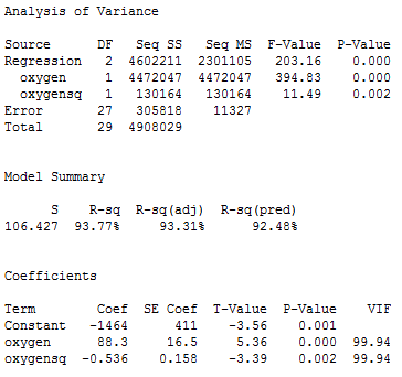
we quickly see that the variance inflation factors for both predictors —oxygen and oxygensq —are very large (99.9 in each case). Is this surprising to you? If you think about it, we've created a correlation by taking the predictor oxygen and squaring it to obtain oxygensq. That is, just by the nature of our model, we have created a "structural multicollinearity."
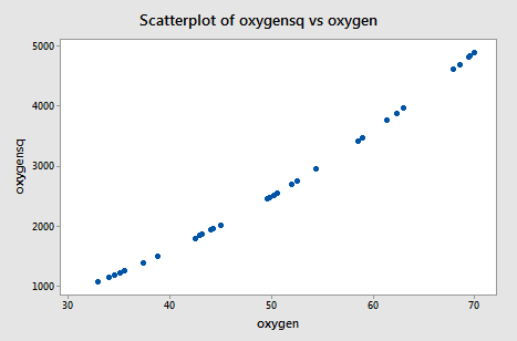
The scatter plot of oxygensq versus oxygen:
![]()
illustrates the intense strength of the correlation that we induced. After all, we just can't get much more correlated than a correlation of r = 0.995!
The neat thing here is that we can reduce the multicollinearity in our data by doing what is known as "centering the predictors." Centering a predictor merely entails subtracting the mean of the predictor values in the data set from each predictor value. For example, the mean of the oxygen values in our data set is 50.64:
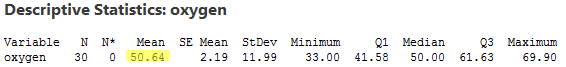
Therefore, in order to center the predictor oxygen, we merely subtract 50.64 from each oxygen value in our data set. Doing so, we obtain the centered predictor, oxcent, say:
| oxygen |
oxcent | oxcentsq |
| 34.6 | -16.04 | 257.282 |
| 45.0 | -5.64 | 31.810 |
| 62.3 | 11.66 | 135.956 |
| 58.9 | 8.26 | 68.228 |
| 42.5 | -8.14 | 66.260 |
| 44.3 | -6.34 | 40.196 |
| 67.9 | 17.26 | 297.908 |
| 58.5 | 7.86 | 61.780 |
| 35.6 | -15.04 | 226.202 |
| 49.6 | -1.04 | 1.082 |
| 33.0 | -17.64 | 311.170 |
For example, 34.6 minus 50.64 is -16.04, and 45.0 minus 50.64 is -5.64, and so on. Now, in order to include the squared oxygen term in our regression model—to allow for curvature in the trend—we square the centered predictor oxcent to obtain oxcentsq. That is, (-16.04)2 = 257.282 and (-5.64)2 = 31.810, and so on.
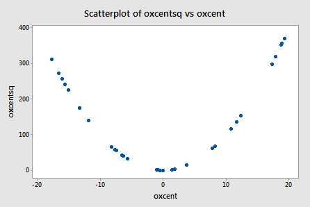
Wow! It really works! The scatter plot of oxcentsq versus oxcent:
![]()
illustrates—by centering the predictors—just how much we've reduced the correlation between the predictor and its square. The correlation has gone from a whopping r = 0.995 to a rather low r = 0.219!
Having centered the predictor oxygen, we must reformulate our quadratic polynomial regression model accordingly. That is, we now formulate our model as:
\[y_i=\beta_{0}^{*}+\beta_{1}^{*}(x_i-\bar{x})+\beta_{11}^{*}(x_i-\bar{x})^{2}+\epsilon_i\]
or alternatively:
\[y_i=\beta_{0}^{*}+\beta_{1}^{*}x_{i}^{*}+\beta_{11}^{*}x_{i}^{*2}+\epsilon_i\]
where:
- yi = amount of immunoglobin in blood (mg), and
- \(x_{i}^{*}=x_i-\bar{x}\) denotes the centered predictor
and the error terms εi are independent, normally distributed and have equal variance σ2. Note that we add asterisks to each of the parameters in order to make it clear that the parameters differ from the parameters in the original model we formulated.
Let's see how we did by centering the predictors and reformulating our model. Recall that —based on our original model —the variance inflation factors for oxygen and oxygensq were 99.9. Now, regressing y = igg on the centered predictors oxcent and oxcentsq:
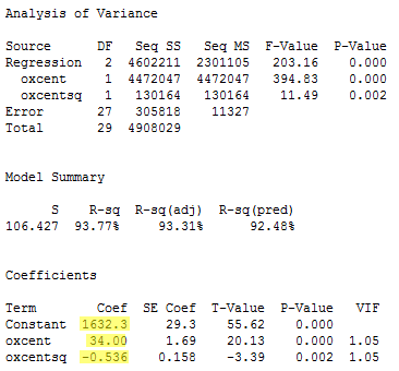
we see that the variance inflation factors have dropped significantly—now they are 1.05 in each case.
Because we reformulated our model based on the centered predictors, the meaning of the parameters must be changed accordingly. Now, the estimated coefficients tell us:
- The estimated coefficient b0 is the predicted response y when the predictor x equals the sample mean of the predictor values.
- The estimated coefficient b1 is the estimated slope of the tangent line at the predictor mean — and, often, it is similar to the estimated slope in the simple linear regression model.
- The estimated coefficient b2 indicates the up/down direction of curve. That is:
- if b2 < 0, then the curve is concave down
- if b2 > 0, then the curve is concave up
So, here, in this example, the estimated coefficient b0 = 1632.3 tells us that a male whose maximal oxygen uptake is 50.64 ml/kg is predicted to have 1632.3 mg of immunoglobin in his blood. And, the estimated coefficient b1 = 34.00 tells us that the when an individual's maximal oxygen uptake is near 50.64 ml/kg, we can expect the individual's immunoglobin to increase by 34.00 mg for every 1 ml/kg increase in maximal oxygen uptake.
As the following plot of the estimated quadratic function suggests:
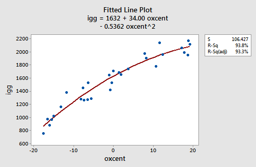
the reformulated regression function appears to describe the trend in the data well. The adjusted R2-value is still 93.3%.
We shouldn't be surprised to see that the estimates of the coefficients in our reformulated polynomial regression model are quite similar to the estimates of the coefficients for the simple linear regression model:
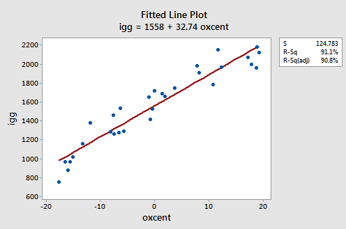
As you can see, the estimated coefficient b1 = 34.00 for the polynomial regression model and b1 = 32.74 for the simple linear regression model. And, the estimated coefficient b0 = 1632 for the polynomial regression model and b0 = 1558 for the simple linear regression model. The similarities in the estimates, of course, arise from the fact that the predictors are nearly uncorrelated and therefore the estimates of the coefficients don't change all that much from model to model.
Now, you might be getting this sense that we're "mucking around with the data" in order to get an answer to our research questions. One way to convince you that we're not is to show you that the two estimated models are algebraically equivalent. That is, if given one form of the estimated model, say the estimated model with the centered predictors:
\[y_i=b_{0}^{*}+b_{1}^{*}x_{i}^{*}+b_{11}^{*}x_{i}^{*2}\]
then, the other form of the estimated model, say the estimated model with the original predictors:
\[y_i=b_{0}+b_{1}x_{i}+b_{11}x_{i}^{2}\]
can be easily obtained. In fact, it can be shown algebraically that the estimated coefficients of the original model equal:
\[\begin{align}
b_{0}&=b_{0}^{*}-b_{1}^{*}\bar{x}+b_{11}^{*}\bar{x}^{2}\\
b_{1}&= b_{1}^{*}-2b_{11}^{*}\bar{x}\\
b_{11}&= b_{11}^{*}\\
\end{align}\]
For example, the estimated regression function for our reformulated model with centered predictors is:
\[\hat{y}_i=1632.3+34.00x_{i}^{*}-0.536x_{i}^{*2}\]
Then, since the mean of the oxygen values in the data set is 50.64:
it can be shown algebraically that the estimated coefficients for the model with the original (uncentered) predictors are:
b0 = 1632.3 - 34.00(50.64) - 0.536(50.64)2 = -1464
b1 = 34.00 - 2(- 0.536)(50.64) = 88.3
b11 = - 0.536
That is, the estimated regression function for our quadratic polynomial model with the original (uncentered) predictors is:
\[\hat{y}_i=-1464+88.3x_{i}-0.536x_{i}^{2}\]
Given the equivalence of the two estimated models, you might ask why we bother to center the predictors. The main reason for centering to correct structural multicollinearity is that low levels of multicollinearity can be helpful in avoiding computational inaccuracies. Specifically, a near-zero determinant of XTX is a potential source of serious roundoff errors in the calculations of the normal equations. Severe multicollinearity has the effect of making this determinant come close to zero. Thus, under severe multicollinearity, the regression coefficients may be subject to large roundoff errors.
Let's use our model to predict the immunoglobin level in the blood of a person whose maximal oxygen uptake is 70 ml/kg. Of course, before we use our model to answer a research question, we should always evaluate it first to make sure it means all of the necessary conditions. The residuals versus fits plot:
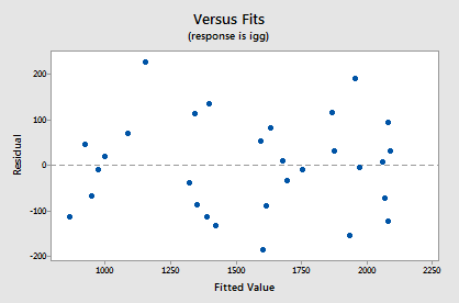
shows a nice horizontal band around the residual = 0 line, suggesting the model fits the data well. It also suggests that the variances of the error terms are equal. And, the normal probability plot:
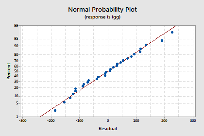
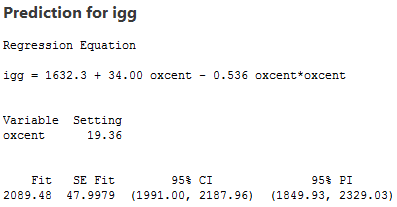
suggests that the error terms are normally distributed. Okay, we're good to go —let's use the model to answer our research question: "What is one's predicted immunoglobin level if the maximal oxygen uptake is 70 ml/kg?"
When making this prediction, you have to remember that we have centered the predictors. That is, if oxygen = 70, then oxcent = 70-50.64 = 19.36. And, if oxcent = 19.36, then oxcentsq = 374.8096. Predicting igg of an individual whose oxcent = 19.36 and oxcentsq = 374.8096, we obtain the following output: