Okay, now that we know the effects that multicollinearity can have on our regression analyses and subsequent conclusions, how do we tell when it exists? That is, how can we tell if multicollinearity is present in our data?

Some of the common methods used for detecting multicollinearity include:

• The analysis exhibits the signs of multicollinearity — such as, estimates of the coefficients vary excessively from model to model.
• The t-tests for each of the individual slopes are non-significant (P > 0.05), but the overall F-test for testing all of the slopes are simultaneously 0 is significant (P < 0.05).
• The correlations among pairs of predictor variables are large.

Looking at correlations only among pairs of predictors, however, is limiting. It is possible that the pairwise correlations are small, and yet a linear dependence exists among three or even more variables, for example, if X₃ = 2X₁ + 5X₂ + error, say. That's why many regression analysts often rely on what are called variance inflation factors (VIF) to help detect multicollinearity.

What is a Variation Inflation Factor?

As the name suggests, a variance inflation factor (VIF) quantifies how much the variance is inflated. But what variance? Recall that we learned previously that the standard errors — and hence the variances — of the estimated coefficients are inflated when multicollinearity exists. A variance inflation factor exists for each of the predictors in a multiple regression model. For example, the variance inflation factor for the estimated regression coefficient b_j —denoted VIF_j —is just the factor by which the variance of b_j is "inflated" by the existence of correlation among the predictor variables in the model.

In particular, the variance inflation factor for the j^th predictor is:

\[VIF_j=\frac{1}{1-R_{j}^{2}}\]

where \(R_{j}^{2}\)  is the R²-value obtained by regressing the j^th predictor on the remaining predictors. 

How do we interpret the variance inflation factors for a regression model? A VIF of 1 means that there is no correlation among the j^th predictor and the remaining predictor variables, and hence the variance of b_j is not inflated at all. The general rule of thumb is that VIFs exceeding 4 warrant further investigation, while VIFs exceeding 10 are signs of serious multicollinearity requiring correction.

An Example

Let's return to the blood pressure data (bloodpress.txt) in which researchers observed the following data on 20 individuals with high blood pressure:

• blood pressure (y = BP, in mm Hg)
• age (x₁ = Age, in years)
• weight (x₂ = Weight, in kg)
• body surface area (x₃ = BSA, in sq m)
• duration of hypertension (x₄ = Dur, in years)
• basal pulse (x₅ = Pulse, in beats per minute)
• stress index (x₆ = Stress)

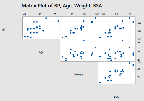
As you may recall, the matrix plot of BP, Age, Weight, and BSA:

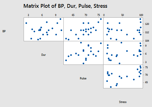
the matrix plot of BP, Dur, Pulse, and Stress:

and the correlation matrix:

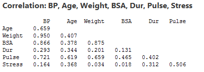
suggest that some of the predictors are at least moderately marginally correlated. For example, body surface area (BSA) and weight are strongly correlated (r = 0.875), and weight and pulse are fairly strongly correlated (r = 0.659). On the other hand, none of the pairwise correlations among age, weight, duration and stress are particularly strong (r < 0.40 in each case).

Regressing y = BP on all six of the predictors, we obtain:

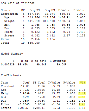
As you can see, three of the variance inflation factors —8.42, 5.33, and 4.41 —are fairly large. The VIF for the predictor Weight, for example, tells us that the variance of the estimated coefficient of Weight is inflated by a factor of 8.42 because Weight is highly correlated with at least one of the other predictors in the model.

For the sake of understanding, let's verify the calculation of the VIF for the predictor Weight. Regressing the predictor x₂ = Weight on the remaining five predictors:

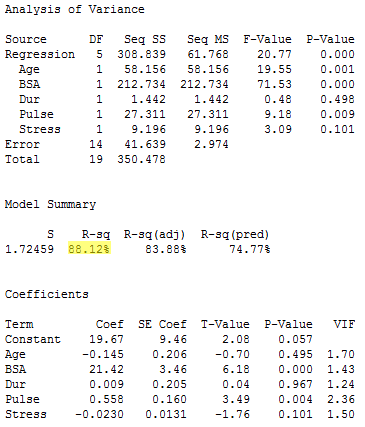
\(R_{Weight}^{2}\) is 88.12% or, in decimal form, 0.8812. Therefore, the variance inflation factor for the estimated coefficient Weight is by definition:

\[VIF_{Weight}=\frac{Var(b_{Weight})}{Var(b_{Weight})_{min}}=\frac{1}{1-R_{Weight}^{2}}=\frac{1}{1-0.8812}=8.42.\]

Again, this variance inflation factor tells us that the variance of the weight coefficient is inflated by a factor of 8.42 because Weight is highly correlated with at least one of the other predictors in the model.

So, what to do? One solution to dealing with multicollinearity is to remove some of the violating predictors from the model. If we review the pairwise correlations again:

we see that the predictors Weight and BSA are highly correlated (r = 0.875). We can choose to remove either predictor from the model. The decision of which one to remove is often a scientific or practical one. For example, if the researchers here are interested in using their final model to predict the blood pressure of future individuals, their choice should be clear. Which of the two measurements — body surface area or weight — do you think would be easier to obtain?! If indeed weight is an easier measurement to obtain than body surface area, then the researchers would be well-advised to remove BSA from the model and leave Weight in the model.

Reviewing again the above pairwise correlations, we see that the predictor Pulse also appears to exhibit fairly strong marginal correlations with several of the predictors, including Age (r = 0.619), Weight (r = 0.659) and Stress (r = 0.506). Therefore, the researchers could also consider removing the predictor Pulse from the model.

Let's see how the researchers would do. Regressing the response y = BP on the four remaining predictors Age, Weight, Duration, and Stress, we obtain:

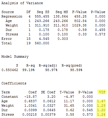
Aha — the remaining variance inflation factors are quite satisfactory! That is, it appears as if hardly any variance inflation remains. Incidentally, in terms of the adjusted R²-value, we did not seem to lose much by dropping the two predictors BSA and Pulse from our model. The adjusted R²-value decreased to only 98.97% from the original adjusted R²-value of 99.44%.