14.2 - Recursive Partitioning
Recursive Partitioning for Classification
Recursive partitioning is a very simple idea for clustering. It is the inverse of hierarchical clustering.
In hierarchical clustering, we start with individual items and cluster those that are closest in some metric. In recursive partitioning, we start with a single cluster and then split into clusters that have the smallest within cluster distances in some metric. When we are doing recursive partitioning for clustering, the "within cluster distance" is just a measure of how homogeneous the cluster is with respect to the classes of the objects in it. For example, a cluster with all the same tissue type is more homogeneous than a cluster with a mix of tissue types.
There are several measures of cluster homogeneity. Denote the proportion of the node coming from type i as \( p(i|node)\) . The most popular homogeneity measure is the Gini index: \(\Sigma_{i,j} p(i|node)p(j|node)\) where i, j are the classes. If all the nodes are homogeneous the Gini index is zero. The impurity index is a similar idea based on information theory.: \(-\Sigma_{i,j} p(i|node) log (p(j|node))\).
For gene expression data, we start with a set of preselected genes and some measure, such as gene expression, for each gene. These may have been selected based on network analysis, or more simply based on a differential expression analysis. We start with a single node(cluster) containing all the samples, and recursively split into increasingly homogeneous clusters. At each step, we select a node to split and split it independently of other nodes and any splits already performed.
The measures on each gene are the splitting variables. For each possible value of each selection variable, we partition the node into two groups - samples above the cut-off or less than or equal the cut-off. The algorithm simply considers all possible splits for all possible variables and selects the variable and split that creates the most homogeneous clusters. (Note that if a variable includes two values say A and B with no values between, then any cut-off between A and B produces the same 2 clusters, so the algorithm only needs to search through a finite number of splits - the midpoints between adjacent observed values.
We stop splitting when the leaves are all pure or have less than r elements (where r is chosen in advance).
Hence this process creates a recursive binary tree.
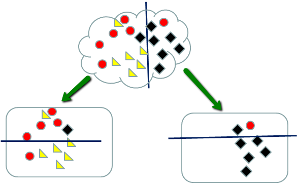
When splitting stops, the samples in each node are classified according to a majority rule. So the left nodes above are declared red (upper) and yellow (lower) leading to 3 misclassified samples. The right nodes are declared either black or red (upper) and black (lower) leading to one misclassified sample.
It is quite easy to overfit when using this method. Overfitting occurs when we fit the noise as well as the signal. In this case, it would mean adding a branch that works well for this particular sample by chance. An overfitted classifier works well with the training sample, but when new data are classified it makes more mistakes than a classifier with few branches.
Determining when to stop splitting is more of an art than a science. It is usually not useful to partition down to single elements as this increases overfitting. Cross-validation, which will be discussed in the next lesson, is often used to help tune the tree selection without over-fitting.
How do you classify a new sample for which the category is unknown? The new sample will have the same set of variables (measured features). You start at the top the tree and "drop" the sample down the tree. The classification for the new sample is the majority type in the terminal node. Sometimes instead of a "hard" classification into a type, the proportion of training samples in the node is used to obtain a probabilistic (fuzzy) classification. If the leaf is homogeneous, the new sample is assigned to that type with probability one. If the leaf is a mixture, then you assign the new sample to each component of the mixture with probability equal to the mixture proportion.
A more recent (and now more popular method) is to use grow multiple trees using random subsets of the data. This is called a "random forest". The final classifier uses all of the tree rules. To classify a new sample, it is dropped down all the trees (following the tree rules). This gives it a final classification by "voting" - each sample is classified into the type obtained from the majority of trees. This consensus method will be discussed in more detail in the lesson on the cross-validation, bootstraps and consensus.
Recursive partitioning bases the split points on each variable, looking for a split that increases the homogeneity of the resulting subsets. If two splits are equally good, the algorithm selects one. The "goodness" of the split does not depend on any measure of distance between the nodes, only the within node homogeneity. All the split points are based on one variable at a time; therefore they are represented by vertical and horizontal partitioning of the scatterplot. We will demonstrate the splitting algorithm using the two most differentially expressed genes as seen below.
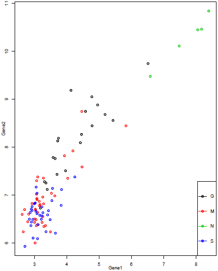
The first split uses gene 2 and splits into two groups based on log2(expression) above or below 7.406.
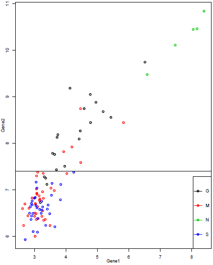
Then the two groups are each split again. They could be split on either gene, but both are split on gene 1. This gives 4 groups:
gene 2 below 7.406, gene 1 above/below 3.35
gene 2 above 7.406, gene 1 above/below 5.6. (note that the "above" group is a bit less homogeneous than it would be with a higher split, but the "below" group is more homogeneous)
The entire tree grown using just these 2 genes is shown below:
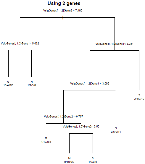
Each of the terminal (leaf) nodes is labeled with the category making up the majority. The numbers below each leaf is the number of samples in G\M\N\S. We can see that none of these leaf nodes is purely one category, so there are lots of misclassified genes. However, we can distinguish reasonably well between the normal and cancerous samples, and between G and the other two cancer types. How well can we do with the 10 best genes? That tree is displayed below:
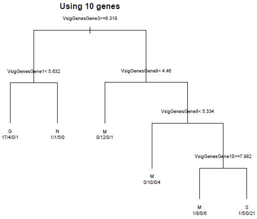
Only 5 of the 10 most differentially expressed genes are used in the classification. We do a bit better than with only two genes, but still have a lot of misclassified genes.
Notice that we have misclassified two tumor samples as normal. We might be less worried about misclassifying the cancer samples among themselves and more worried about misclassifying them as normal, since a classification as cancerous will likely lead to further testing. A weighting of the classification cost, to make it more costly to misclassify cancer samples can provide a classification that does better at separating out the normal from cancer samples. This is readily done by providing misclassification weights.

