14.4 - Support Vector Machine
The idea behind the basic support vector machine (SVM) is similar to LDA - find a hyperplane separating the classes. In LDA, the separating hyperplane separates the means of the samples in each class, which is suitable when the data are sitting inside an ellipsoid or other convex set. However, intuitively what we really want is a rule that separates the samples in the different classes which appear to be closest. When the classes are separable (i.e. can be separated by a hyperplane without misclassification), the support vector machine (SVM) finds the hyperplane that maximizes the minimum distance from the hyperplane to the nearest point in each set. The nearest points are called the support vectors.
In discriminant analysis, the assumption is that the samples cluster more tightly around the mean of the within class distribution. Using this method the focus is on separating the ellipsoids containing the bulk of the samples within each class.
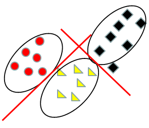
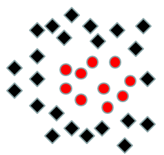
Using a SVM, the focus is on separating the closest points in different classes. The first step is to determine which point or points are closest to the other classes. These points are called support vectors because each sample is described by its vector of values on the genes (e.g. expression values). After identifying the support vectors (circled below) for each pair of classes we compute the separating hyperplane by computing the shortest distance from each support vector to the line. We then select the line the maximizes the sum of distances. If it is impossible to completely separate the classes, then a negative penalty is applied for misclassification - the selected line then maximizes the sum of distances plus penalty, which balances the distances from the support vectors to the line and the misclassifications.
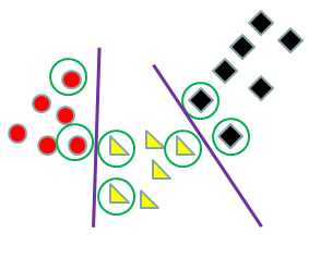
The separating hyperplane used in LDA is sensitive to all the data in each class because you are using the entire ellipse of data and its center. The separating hyperplane used in SVM is sensitive only to the data on the boundary which provides computational savings and makes it more to robust outliers.
This is how it is applied:
Suppose the data vector for the ith sample is \(x_i\), which is the expression vector for several genes. Also, suppose we have only 2 classes denoted by \(y_i= +/- 1\). The hyperplane is defined by a vector W and a scalar b such that for all i.
\(y_i(x_i'W+b)-1\ge 0\) for all i with equality for the support vectors and \(||W||\) is minimal. After computing W and b using the training set, new samples are classified by determining the value of y satisfying the inequality.
If the clusters overlap, the "obvious" extension is to find the hyperplane that minimizes the distance between the main samples and the hyperplane, while penalizing for misclassified samples.
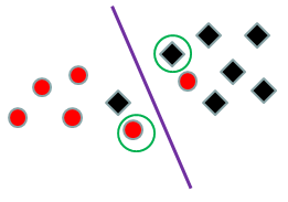
This is the solution to the optimization problem: \(y_i(x_i'W+b)-1+z_i \ge 0)\) for all i with equality for the support vectors where all \(z_i ≥ 0\) and \(||W|| + C\Sigma_i z_i\) is minimal for some C.
The idea is that some points can be one the wrong side of the separating hyperplane, but there is a penalty for each misclassification. The hyperplane is now found by minimizing a criterion that still separates the support vectors as much as possible in this orthogonal direction, but also minimizes the number of misclassifications.
It is not clear that SVM does much better than linear discriminant analysis when the groups are actually elliptical. When the groups are not elliptical because of outliers SVM does better because the criterion is only sensitive to the boundaries and not sensitive to the entire shape. However, like LDA, SVM requires groups that can be separated by planes. Neither method will do well for an example like the one below. However, there is a method called the kernel method (sometimes called the kernel trick) that works for more general examples.
The idea is simple - the implementation is very clever.
Suppose that we suspected that the clusters were in concentric circles (or spheres) as seen above. If we designate the very center of the points as the origin, we can compute the distance from each point to the center as a new variable. In this case, the clusters separate very nicely on the radius, creating a circular boundary.
The general idea is to add more variables that are nonlinear functions of the original variables until we have enough dimensions to separate the groups.
The kernel trick uses the fact that for both LDA and SVM, only the dot product of the data vectors \(x_i'x_j\) are used in the computations. Lets call \(K(x_i,x_j)=x_i'x_j\). We replace $K$ with a more general function called a kernel function and use \(K(x_i,x_j)\) as if it were the dot product in our algorithm. (For those who are more mathematically inclined, the kernel function needs to be positive definite, and we will actually be using the dot product in the basis described by its eigenfunctions.)
The most popular kernels are the radial kernel and polynomial kernel. The radial kernel (sometimes called the Gaussian kernel) is \(k(x_i, x_j)= \text{exp}(-||x_i-x_j||^2/2\sigma^2)\).
Here is an animation that shows how "kernel" SVM works with the concentric circles using the radial kernel.
Here is another example of essentially the same problem using a polynomial kernel instead of Normal densities. \(k(x_i, x_j)=(x_i'x_j+1)^2\).
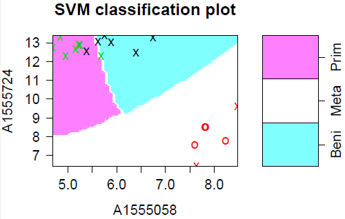
The plot below shows the results of ordinary (linear) SVM on our cancer data. I believe the blue "tail" is an artifact of the plotting routine - the boundaries between the groups should be straight lines. The data points marked with "X" are the support points - there are a lot of them because the data are so strung out.
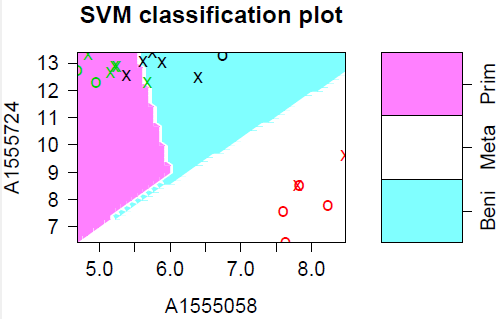
I also used SVM with the radial kernel (below). The plot looks nicer, but there are actually more support points (15 instead of 12) and the same 2 samples are misclassified.