Printer-friendly version

The permutation test can be used to test whether two populations have the same mean both with independent and paired samples, but it is difficult to use all the samples if some are independent and others are paired.  The t-test, which is based on statistical theory, is also suitable for either independent or paired samples, but not a mix.  However, the statistical theory can be extended to handle a mixed sample.  This makes t-tests and their generalizations the basis for much of the work in differential expression analysis.

The t-test uses an approximation to the sampling distribution of the difference in sample means based on the Central Limit Theorem, which ensures that for sufficiently large samples, the sampling distribution will be very close to Normal.  The mean of the sampling distribution will be the difference in population means, and the variance of the sampling distribution will be the standard error of the difference in sample means.  This approximation works quite well even for small samples (say sample sizes of 10 for both conditions) unless the data are highly skewed.  For gene expression data measured on microarrays, taking logarithms of expression usually reduces skewness enough for this approximation to work well. 

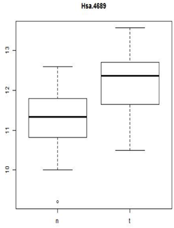
In this case our two conditions are the normal tissue samples and the tumor  tissue samples. We estimate the population means by using the sample means \(\bar{X}\) for normal and \(\bar{Y}\) for tumor.  We estimate the the population variances using the sample variances \(S^2_X\) and \(S^2_Y\). For the 40 independent samples,  we plug the sample variances into the formula for the standard error of the difference in sample means \(\sqrt{\frac{S^2_X}{n_X}+\frac{S^2_Y}{n_Y}}\) where \(n_X\) and \(n_Y\) are the sample sizes. 

Now, if the null hypothesis was true we expect that \(\bar{X} - \bar{Y}\) would be close to zero.  Just as with the permutation test, "close" is relative to the sampling distribution.  And we have an estimate of the SD of the sampling distribution. Statistical theory then tells us that if the underlying populations are close to Normal, are independent and there is no difference in population means, then

\[ t*=\frac{\bar{X} - \bar{Y}}{\sqrt{\frac{S^2_X}{n_X}+\frac{S^2_Y}{n_Y}}}\]

has a Student-t distribution.

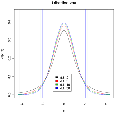
Density histograms of t-distribution for different degrees of freedom.
95% of the sample should yield t values between the vertical lines of the given color.

Student-t is actually a family of distributions defined by a parameter called the degrees of freedom or d.f.  The degrees of freedom have to do with the error in estimating variance using the sample variance instead of knowing exactly what it is from the population. When there are infinite d.f, we get the Normal distribution.  The larger the d.f. the higher the peak at 0 and the small the percentage of the population which are less than -3 or greater than 3. In the plot above, 95% of the population designated by the color are between vertical bars of the same color.  With 30 d.f. the bars are at +/- 2.04.  So an unusual value of t would be anything with absolute value greater than 2.04.  Similarly, for 2 d.f. the bars are at +/- 4.3. The brilliance of the t-test is that if the null hypothesis is true then the two sample means and variances and the sample sizes are sufficient to compute the t-value and determine the associated p-value.

In the special case when X and Y have the same population variance, we use a pooled variance estimator and the d.f. are exactly \( (n_X-1)+(n_Y-1)\).  In general, however, the population variances are not the same and we use the individual variance estimates as given above.  In that case, a fairly complex formula is used to estimate the d.f. and the d.f. may be fractional.  

When the t-value is typical (i.e. near the center of the distribution), it does not provide evidence against the null hypothesis.  I.e. if the null hypothesis is true, then t-values of the observed size readily arise by chance- the difference in sample means is small enough to arise due to measurement and biological variability between samples.

When the population means are not equal, the distribution of t* is shifted by about \(\frac{\mu_X - \mu_Y}{\sqrt{\frac{\sigma^2_X}{n_X}+\frac{\sigma^2_Y}{n_Y}}}\), so that t* is more likely to be in the left tail if  \(\mu_X < \mu_Y\) (blue histogram)  and in the right tail if \(\mu_X > \mu_Y\) (red histogram) and therefore to be an unusual value under the null hypothesis of no difference in means (black histogram).

P-values and d.f.

Usually after computing t*, we convert it to a p-value. Suppose we observe the t-value indicated on the graph with the red arrow. Remember, the p-value is the percentage of the histogram that is more extreme, everything farther from the center of the observed t-value and its reflection designated by the two purple arrows.

We focus on the black and the blue curves. Considering the observed t, is it more surprising if you have 2 degrees of freedom or 30 degrees of freedom?

The degree of "surprise" is measured by the percentage of the sampling distribution of t* (when the null hypothesis is true)  that would be more extreme than the observed value - i.e. the area under the histogram from the observed t value out to the left and its reflection out to the right. The blue distribution is lower than the black, so there is less room or a smaller percentage of the sampling distribution under the blue distribution then there is under the black. Therefore, it is more surprising if you have 30 degrees of freedom than if you have 2 degrees of freedom. Remember, the degrees of freedom comes from the the two sample sizes. So, for any value of t* that is not exactly zero, the value is more surprising with larger sample sizes. We expect with small sample sizes that \(\bar{X}-\bar{Y}\) might be quite variable and as well the estimate of the sample variances might also be poor, so there is a lot of variability in t*. But in large samples the sample estimates should be closer to the true values.  So if there's no difference between gene expression in the normal tissue samples compared to the tumor tissue samples we expect t* to be close to zero in larger samples than in smaller samples.

Often what we say that there is a significant difference if the p-value is less than .05, i.e. the percent of samples that would be more extreme is less than .05. The vertical lines in the histogram show this.  The observed t* is significant at p<0.05 for 10 and 30 d.f. but not for 5 and 2 d.f.

Very occasionally we know in advance whether we should be expecting things to be over expressed or under expressed in a certain tissue. In these cases we would only use a one tailed test. Usually, however, we are testing both over and under-expression and use both tails to compute the p-value.

We could compute t* on a calculator and look up the p-value on a t-table, but it is easier to use R.  

Results of Welch Two Sample t-test data: 

t = -3.9224, df = 37.999, p-value = 0.0003553

95 percent confidence interval:   (-1.3866216,-0.4425592)

The p-value for our normal versus tumor tissue samples is 0.0003. This is surprising! This is the probability of seeing something this extreme or more if there is no difference in mean expression.  We either got a very unusual sample or the null hypothesis is false and mean expression is higher in the tumor tissue.

The confidence interval is the set of all possible differences  in population means for which the observed value of t* would NOT be surprising. The confidence interval tells us that plausible values of the difference in population means is somewhere between -1.39 and -0.44.

We should notice is that statistical significance is not the same as practical significance.  Biologists often target 2-fold expression differences as the minimum for biological relevance (although just like p<0.05 for statistical significance, this is just a rule of thumb).  2-fold is the same as +/-1 on the log2 scale.  In the current example, the observed difference in means is 11.339-12.186=-0.848 which might not be considered biologically significant.

The difference between statistical and biological significance is a criticism of this type of testing. The reason for this is that in the denominator of the test there are quantities that are divided by the sample sizes. So, if the sample sizes are really big, the denominator becomes very small and  tiny differences in the means are going to be statistically significant. 

Some Notes

1.Biologists usually twofold difference in expression to be biologically significant (especially if it is also statistically significant). What about smaller differences such as 5-% or 10%? Is this difference biologically significant?  In any study we will need to combine the evidence with the current data with evidence from previous studies to come up with biological inferences and new hypotheses.

2. The t-test that we use was called Welch's t-test. Welch's t-test allows the two populations to have different spreads. There is another form of the test which where we assume the two populations have about the same spread. This may not be very realistic for  normal and tumor tissue samples. Gene expression in tumor tissues may be much more spread out than in normal tissue. In fact, in a lot of situations when we are looking at something versus the control, the control has lower variance.  Fortunately, the t-test is quite robust to the equal variance assumption unless the differences in expression are very large or the difference in sample sizes is very large.

3. We do need to be careful about independence. 

4. We usually use the log2(expression) which generally helps to equalize variance between the two populations (variance stabilizing) and improves Normality of the underlying populations.