WQD.2 - Multiple Regression
Sample R code for
Multiple Regression
Linear regression is fitted to the Training data.
Model I: All predictors in the model
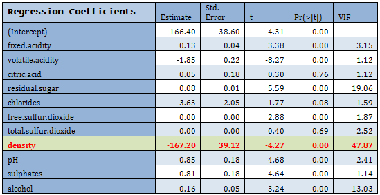
For extremely high VIF density was removed from the model. There are other predictors with high VIF, but they were not removed at this step.
Model II: After removal of density VIFs improved
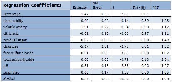
Not all predictors are significant. A forward selection method is employed to build a working model. The sample R output follows:
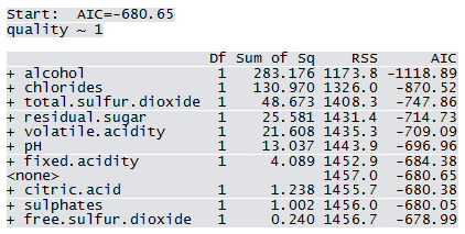
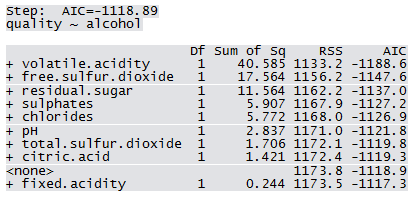
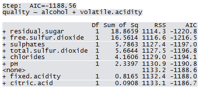
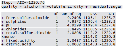
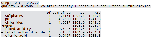
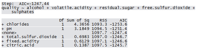
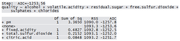
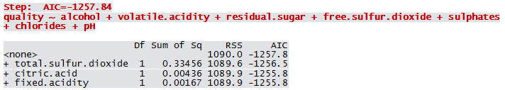
Model III: Working model

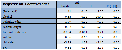
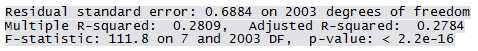
Sample R output:
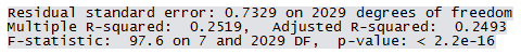
Note that multiple R2 is 25%. Regression diagnostics are examined for possible improvement of the model.
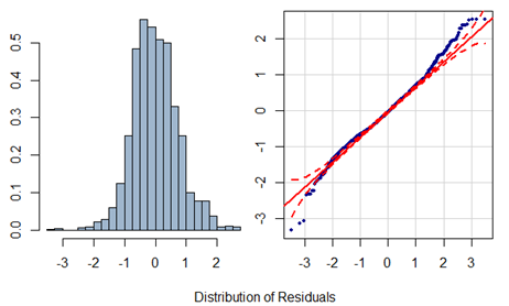
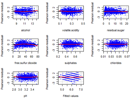
Residuals have an approximately symmetric distribution but there seems to be outliers at both ends. Partial residual plots are given below. Note the pattern in the fitted value plot. Since the response actually takes only integer values but has been assumed to be continuous, such pattern arises.
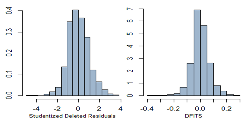
Outliers and leverage points are identified through the following:
- Studentized deleted residuals (a point is outlier if residual is outside of [-3, 3] limits
- DFITS (a point is outlier if residual is outside of [-1, 1] limits
- Cook’s distance
All three plots are given below. Note that no point is identified as outlier with DFITS value.
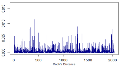
Only 26 points are identified as outliers according to the above criteria. A final model is fit after eliminating these points and a slight improvement in the R2 value is noted.
Model IV: Final model
Sample R output:
Application of this model on test data gives sum of square of differences between the actual response and predicted response to be 1196.205 whereas sum of square of deviations of actual response is 1554.754. Ratio of these two may be taken as the ratio of Error sum of squares and total sum of squares. Hence a measure similar to that of R2 may be computed as 1 – 1196.205/1554.754 = 0.2306.

