Example 16-2 Section
Let \(X\) equal the IQ of a randomly selected American. Assume \(X\sim N(100, 16^2)\). What is the probability that a randomly selected American has an IQ below 90?
Solution
As is the case with all continuous distributions, finding the probability involves finding the area under the curve and to the left of the line \(x=90\):
That is:
\(P(X \leq 90)=F(90)=\int^{90}_{-\infty} \dfrac{1}{16\sqrt{2\pi}}\text{exp}\left\{-\dfrac{1}{2}\left(\dfrac{x-100}{16}\right)^2\right\} dx\)
There's just one problem... it is not possible to integrate the normal p.d.f. That is, no simple expression exists for the antiderivative. We can only approximate the integral using numerical analysis techniques. So, all we need to do is find a normal probability table for a normal distribution with mean \(\mu=100\) and standard deviation \(\sigma=16\). Aw, geez, there'd have to be an infinite number of normal probability tables. That strategy isn't going to work! Aha! The cumulative probabilities have been tabled for the \(N(0,1)\) distribution. All we need to do is transform our \(N(100, 16^2)\) distribution to a \(N(0, 1)\) distribution and then use the cumulative probability table for the \(N(0,1)\) distribution to calculate our desired probability. The theorem that follows tells us how to make the necessary transformation.
If \(X\sim N(\mu, \sigma^2)\), then:
\(Z=\dfrac{X-\mu}{\sigma}\)
follows the \(N(0,1)\) distribution, which is called the standardized (or standard) normal distribution.
Proof
We need to show that the random variable \(Z\) follows a \(N(0,1)\) distribution. So, let's find the cumulative distribution function \(F(z)\), which is also incidentally referred to as \(\Phi(z)\) in the standard normal case (that's the greek letter phi, read "fee"):
\(F(z)=\Phi(z)=P(Z\leq z)=P \left(\dfrac{X-\mu}{\sigma} \leq z \right)\)
which, by rearranging and using the normal p.d.f., equals:
\(F(z)=P(X\leq \mu+z\sigma)=\int^{\mu+z\sigma}_{-\infty} \dfrac{1}{\sigma \sqrt{2\pi}} \text{exp}\left\{-\dfrac{1}{2} \left(\dfrac{x-\mu}{\sigma}\right)^2\right\} \)
To perform the integration, let's use the change of variable technique with:
\(w=\dfrac{x-\mu}{\sigma}\)
so that:
\(x = \sigma(w) + \mu \) and \(dx = \sigma dw\)
Now for the endpoints of the integral: if \(x=-\infty\), then \(w\) also equals \(-\infty\); and if \(x=\mu+z\sigma\), then \(w=\frac{\mu+z\sigma -\mu}{\sigma}\). Therefore, upon making all of the substitutions for \(x, w\), and \(dx\), our integration looks like this:
\(F(z)=\int^z_{-\infty}\dfrac{1}{\sigma \sqrt{2\pi}} \text{exp}\left\{-\dfrac{1}{2} w^2\right\} \sigma dw\)
And since the \(\sigma\) in the denominator cancels out the \(\sigma\) in the numerator, we get:
\(F(z)=\int^z_{-\infty}\dfrac{1}{\sqrt{2\pi}} \text{exp}\left\{-\dfrac{1}{2} w^2\right\} dw\)
We should now recognize that as the cumulative distribution of a normal random variable with mean \(\mu=0\) and standard deviation \(\sigma=1\). Our proof is complete.
The theorem leads us to the following strategy for finding probabilities \(P(z<X<b)\) when \(a\) and \(b\) are constants, and \(X\) is a normal random variable with mean \(\mu\) and standard deviation \(\sigma\):
-
1) Specify the desired probability in terms of \(X\).
-
2) Transform \(X, a\), and \(b\), by:
\(Z=\dfrac{X-\mu}{\sigma}\)
-
3) Use the standard normal \(N(0,1)\) table, typically referred to as the \(Z\)-table, to find the desired probability.
Reading \(Z\)-tables Section
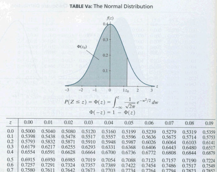
Standard normal, or \(Z\)-tables, can take a number of different forms. There are two standard normal tables, Table Va and Table Vb, in the back of our textbook. Table Va gives the cumulative probabilities for \(Z\)-values, to two decimal places, between 0.00 and 3.09. Here's what the top of Table Va looks like:
\begin{aligned} P(Z \leq z)=& \Phi(z)=\int_{-\infty}^{z} \frac{1}{\sqrt{2 \pi}} e^{-w^{2} / 2} d w \\ \Phi(-z) &=1-\Phi(z) \end{aligned}
| z | 0.00 | 0.01 | 0.02 | 0.03 | 0.04 | 0.05 | 0.06 | 0.07 | 0.08 | 0.09 |
|---|---|---|---|---|---|---|---|---|---|---|
| 0.0 | 0.5000 | 0.5040 | 0.5080 | 0.5120 | 0.5160 | 0.5199 | 0.5239 | 0.5279 | 0.5319 | 0.5359 |
| 0.1 | 0.5398 | 0.5438 | 0.5478 | 0.5517 | 0.5557 | 0.5596 | 0.5636 | 0.5675 | 0.5714 | 0.5753 |
| 0.2 | 0.5793 | 0.5832 | 0.5871 | 0.5910 | 0.5948 | 0.5987 | 0.6026 | 0.6064 | 0.6103 | 0.6141 |
| 0.3 | 0.6179 | 0.6217 | 0.6255 | 0.6293 | 0.6310 | 0.6368 | 0.6406 | 0.6443 | 0.6480 | 0.6517 |
| 0.4 | 0.6554 | 0.6591 | 0.6628 | 0.6664 | 0.6700 | 0.6736 | 0.6772 | 0.6808 | 0.6844 | 0.6879 |

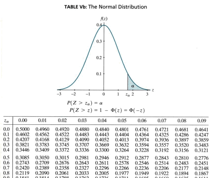
For example, you could use Table Va to find probabilities such as \(P(Z\le 0.01), P(Z\le 1.23)\), or \(P(Z\le 2.98)\). Table Vb, on the other hand, gives probabilities in the upper tail of the standard normal distribution. Here's what the top of Table Vb looks like:
\(P(Z > z_\alpha) = \alpha \)
\(P(Z > z) = 1 - \Phi(z) = \Phi(-z)\)
| \(z_\alpha\) | 0.00 | 0.01 | 0.02 | 0.03 | 0.04 | 0.05 | 0.06 | 0.07 | 0.08 | 0.09 |
|---|---|---|---|---|---|---|---|---|---|---|
| 0.0 | 0.5000 | 0.4960 | 0.4920 | 0.4880 | 0.4840 | 0.4801 | 0.4761 | 0.4721 | 0.4681 | 0.4641 |
| 0.1 | 0.4602 | 0.4562 | 0.4522 | 0.4483 | 0.4443 | 0.4404 | 0.4364 | 0.4325 | 0.4286 | 0.4247 |
| 0.2 | 0.4207 | 0.4168 | 0.4129 | 0.4090 | 0.4520 | 0.4013 | 0.3974 | 0.3936 | 0.3897 | 0.3859 |
| 0.3 | 0.3821 | 0.3783 | 0.3745 | 0.3707 | 0.3669 | 0.3632 | 0.3594 | 0.3570 | 0.3557 | 0.3483 |
| 0.4 | 0.3446 | 0.3409 | 0.3372 | 0.3336 | 0.3300 | 0.3264 | 0.3228 | 0.3192 | 0.3192 | 0.3121 |

That is, for \(Z\)-values, to two decimal places, between 0.00 and 3.49, we can use Table Vb to find probabilities such as \(P(Z>0.12), P(Z>1.96)\), and \(P(Z>3.32)\).
Now, we just need to learn how to read the probabilities off of each of the tables. First Table Va:
And, then Table Vb:
Now we know how to read the given \(Z\)-tables. Now, we just need to work with some real examples to see that finding probabilities associated with a normal random variable usually involves rewriting the problems just a bit in order to get them to "fit" with the available \(Z\)-tables.
Example 16-2 Continued Section
Let \(X\) equal the IQ of a randomly selected American. Assume \(X\sim N(100, 16^2)\). What is the probability that a randomly selected American has an IQ below 90?
Answer
Whenever I am faced with finding a normal probability, I always always always draw a picture of the probability I am trying to find. Then, the problem usually just solves itself... oh, how we wish:
So, we just found that the desired probability, that is, that the probability that a randomly selected American has an IQ below 90 is 0.2643. (If you haven't already, you might want to make sure that you can independently read that probability off of Table Vb.)
Now, although I used Table Vb in finding our desired probability, it is worth mentioning that I could have alternatively used Table Va. How's that? Well:
\(P(X<90)=P(Z<-0.63)=P(Z>0.63)=1-P(Z<0.63)\)
where the first equality comes from the transformation from \(X\) to \(Z\), the second equality comes from the symmetry of the normal distribution, and the third equality comes from the rule of complementary events. Using Table Va to look up \(P(Z<0.63)\), we get 0.7357. Therefore,
\(P(X<90)=1-P(Z<0.63)=1-0.7357=0.2643\)
We should, of course, be reassured that our logic produced the same answer regardless of the method used! That's always a good thing!
What is the probability that a randomly selected American has an IQ above 140?
Answer
Again, I am going to solve this problem by drawing a picture:
So, we just found that the desired probability, that is, that the probability that a randomly selected American has an IQ above 140 is 0.0062. (Again, if you haven't already, you might want to make sure that you can independently read that probability off of Table Vb.)
We again could have alternatively used Table Va to find our desired probability:
\(P(X>140)=P(Z>2.50)=1-P(Z<2.50\)
where the first equality comes from the transformation from \(X\) to \(Z\), and the second equality comes from the rule of complementary events. Using Table Va to look up \(P(Z<2.5)\), we get 0.9938. Therefore,
\(P(X>140)=1-P(Z<2.50)=1-0.9938=0.0062\)
Again, we arrived at the same answer using two different methods.
What is the probability that a randomly selected American has an IQ between 92 and 114?
Answer
Again, I am going to solve this problem by drawing a picture:
So, we just found that the desired probability, that is, that the probability that a randomly selected American has an IQ between 92 and 114 is 0.5021. (Again, if you haven't already, you might want to make sure that you can independently read the probabilities that we used to get the answer from Tables Va and Vb.)
The previous three examples have illustrated each of the three possible normal probabilities you could be faced with finding —below some number, above some number, and between two numbers. Once you have mastered each case, then you should be able to find any normal probability when asked.