Now that we have an intuitive feel for the Central Limit Theorem, let's use it in two different examples. In the first example, we use the Central Limit Theorem to describe how the sample mean behaves, and then use that behavior to calculate a probability. In the second example, we take a look at the most common use of the CLT, namely to use the theorem to test a claim.
Example 27-3 Section

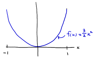
Take a random sample of size \(n=15\) from a distribution whose probability density function is:
\(f(x)=\dfrac{3}{2} x^2\)
for \(-1<x<1\). What is the probability that the sample mean falls between \(-\frac{2}{5}\) and \(\frac{1}{5}\)?
Solution
The expected value of the random variable \(X\) is 0, as the following calculation illustrates:
\(\mu=E(X)=\int^1_{-1} x \cdot \dfrac{3}{2} x^2dx=\dfrac{3}{2} \int^1_{-1}x^3dx=\dfrac{3}{2} \left[\dfrac{x^4}{4}\right]^{x=1}_{x=-1}=\dfrac{3}{2} \left(\dfrac{1}{4}-\dfrac{1}{4} \right)=0\)
The variance of the random variable \(X\) is \(\frac{3}{5}\), as the following calculation illustrates:
\(\sigma^2=E(X-\mu)^2=\int^1_{-1} (x-0)^2 \dfrac{3}{2} x^2dx=\dfrac{3}{2} \int^1_{-1}x^4dx=\dfrac{3}{2} \left[\dfrac{x^5}{5}\right]^{x=1}_{x=-1}=\dfrac{3}{2} \left(\dfrac{1}{5}+\dfrac{1}{5} \right)=\dfrac{3}{5}\)
Therefore, the CLT tells us that the sample mean \(\bar{X}\) is approximately normal with mean:
\(E(\bar{X})=\mu_{\bar{X}}=\mu=0\)
and variance:
\(Var(\bar{X})=\sigma^2_{\bar{X}}=\dfrac{\sigma^2}{n}=\dfrac{3/5}{15}=\dfrac{3}{75}=\dfrac{1}{25}\)
Therefore the standard deviation of \(\bar{X}\) is \(\frac{1}{5}\). Drawing a picture of the desired probability:
we see that:
\(P(-2/5<\bar{X}<1/5)=P(-2<Z<1)\)
Therefore, using the standard normal table, we get:
\(P(-2/5<\bar{X}<1/5)=P(Z<1)-P(Z<-2)=0.8413-0.0228=0.8185\)
That is, there is an 81.85% chance that a random sample of size 15 from the given distribution will yield a sample mean between \(-\frac{2}{5}\) and \(\frac{1}{5}\).
Example 27-4 Section

Let \(X_i\) denote the waiting time (in minutes) for the \(i^{th}\) customer. An assistant manager claims that \(\mu\), the average waiting time of the entire population of customers, is 2 minutes. The manager doesn't believe his assistant's claim, so he observes a random sample of 36 customers. The average waiting time for the 36 customers is 3.2 minutes. Should the manager reject his assistant's claim (... and fire him)?
Solution
It is reasonable to assume that \(X_i\) is an exponential random variable. And, based on the assistant manager's claim, the mean of \(X_i\) is:
\(\mu=\theta=2\).
Therefore, knowing what we know about exponential random variables, the variance of \(X_i\) is:
\(\sigma^2=\theta^2=2^2=4\).
Now, we need to know, if the mean \(\mu\) really is 2, as the assistant manager claims, what is the probability that the manager would obtain a sample mean as large as (or larger than) 3.2 minutes? Well, the Central Limit Theorem tells us that the sample mean \(\bar{X}\) is approximately normally distributed with mean:
\(\mu_{\bar{X}}=2\)
and variance:
\(\sigma^2_{\bar{X}}=\dfrac{\sigma^2}{n}=\dfrac{4}{36}=\dfrac{1}{9}\)
Here's a picture, then, of the normal probability that we need to determine:
\(z = \dfrac{3.2 - 2}{\sqrt{\frac{1}{9}}} = 3.6\)
That is:
\(P(\bar{X}>3.2)=P(Z>3.6)\)
The \(Z\) value in this case is so extreme that the table in the back of our text book can't help us find the desired probability. But, using statistical software, such as Minitab, we can determine that:
\(P(\bar{X}>3.2)=P(Z>3.6)=0.00016\)
That is, if the population mean \(\mu\) really is 2, then there is only a 16/100,000 chance (0.016%) of getting such a large sample mean. It would be quite reasonable, therefore, for the manager to reject his assistant's claim that the mean \(\mu\) is 2. The manager should feel comfortable concluding that the population mean \(\mu\) really is greater than 2. We will leave it up to him to decide whether or not he should fire his assistant!
By the way, this is the kind of example that we'll see when we study hypothesis testing in Stat 415. In general, in the process of performing a hypothesis test, someone makes a claim (the assistant, in this case), and someone collects and uses the data (the manager, in this case) to make a decision about the validity of the claim. It just so happens to be that we used the CLT in this example to help us make a decision about the assistant's claim.