10.1 - Hierarchical Clustering
Hierarchical clustering is set of methods that recursively cluster two items at a time. There are basically two different types of algorithms, agglomerative and partitioning. In partitioning algorithms, the entire set of items starts in a cluster which is partitioned into two more homogeneous clusters. Then the algorithm restarts with each of the new clusters, partitioning each into more homogeneous clusters until each cluster contains only identical items (possibly only 1 item). If there is time towards the end of the course we may discuss partitioning algorithms.
In agglomerative algorithms, each item starts in its own cluster and the two most similar items are then clustered. You continue accumulating the most similiar items or clusters together two at a time until there is one cluster. For both types of algorithms, the clusters at each step can be displayed in a dendrogram as we have seen with our microarray and RNA-seq data.
Agglomerative Process
- Choose a distance function for items \(d(x_i, x_j)\)
- Choose a distance function for clusters \(D(C_i, C_j)\) - for clusters formed by just one point, D should reduce to d.
- Start from N clusters, each containing one item. Then, at each iteration:
- a) using the current matrix of cluster distances, find two closest clusters.
- b) update the list of clusters by merging the two closest.
- c) update the matrix of cluster distances accordingly
- Repeat until all items are joined in one cluster.
This is called a greedy algorithm. It looks at only the current state and does the best it can at that stage and does not look ahead to see whether another choice would be better in the long run. If you join two items into the same group early on you cannot determine if a cluster later develops that is actually closer to one of the items. For this reason, you never get to 'shuffle' and put an item back into a better group.
A problem with the algorithm occurs when there are two pairs that could be merged at a particular stage. Only one pair is merged - usually the pair that is first in the data matrix. After this pair is merged the distance matrix is updated, and it is possible that the second pair is no longer closest. If you had picked the other pair first, you could get a different clustering sequence. This is typically not a big problem but could be if it happens early on. The only way to see if this has happened, is to shuffle the items and redo the clustering method to see if you get a different result.
Distance Measures
One of the problems with any kind of clustering method is that clusters are always created ubt may not always have meaning. One way to think about this is what would happen if we tried to cluster people in a given room. We could cluster people in any number of ways and these would all be valid clusters. We could cluster by:
- gender
- profession
- country of origin
- height
These are all valid clusterings but they have different meanings. The importance of the clustering depends on whether the clustering criterion is associated with the phenomenon under study.
In biological studies, we often don't know what aspects of the data are important. We have to set a distance measure that makes sense for our study. A set of commonly used distance measures is in the table below. The vectors x and y are either samples, in which case their components are the expression measure for each feature, or features, in which case their components are the expression of the feature either in each sample or (better) the mean expression in each treatment.
|
'euclidean': |
Usual square distance between the two vectors (2 norm). |
| 'maximum': | Maximum distance between two components of x and y (supremum norm) |
| 'manhattan': | Absolute distance between the two vectors (1 norm). |
| 'canberra': |
\(\sum(|x_i - y_i| / |x_i + y_i|)\). Terms with zero numerator and denominator are omitted from the sum and treated as if the values were missing. |
| 'minkowski': |
The p norm, the pth root of the sum of the pth powers of the differences of the components. |
| 'correlation': |
1 - r where r is the Pearson or Spearman correlation |
| 'absolute correlation': |
1 - | r | |
For most common hierarchical clustering software, the default distance measure is the Euclidean distance. This is the square root of the sum of the square differences. However, for gene expression, correlation distance is often used. The distance between two vectors is 0 when they are perfectly correlated. The absolute correlation distance may be used when we consider genes to be close to one another either when they go up and down together or in opposition i.e. wherever one gene over-expresses, the other gene under-expresses and vice versa. Absolute correlation distance is unlikely to be a sensible distance when clustering samples. R has a function that computes distances between the columns of matrices and offers many different distance functions.
To understand the differences between some of the distance measures, take a look at the graphs below, each showing the expression pattern of a particular gene (black) versus another gene on the log2 scale on 25 treatments (or 25 samples). Which gene is closest expression pattern to the black gene?
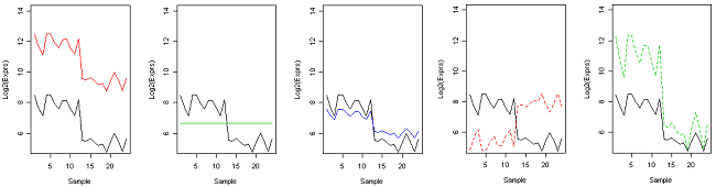
Our visual assessment is closest to Euclidean distance - we tend to focus on the differences between the expression values, which might consider the solid red gene to be the furthest, and the solid blue to be the closest. However, in clustering gene expression, we are more interested in the pattern than the overall mean expression.
If you subtract the mean, which is called centering, you find that you can't even see the difference between the solid red and black genes. The geen, blue and dashed red genes already had the same mean as the black gene and were not affected by centering. The similarity between the dashed green and black genes are now higher.
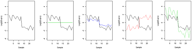
Centered gene expression
Now suppose we take the z-score of expression. The Euclidean distance of the z-scores is the same as correlation distance. z-scores are computed from the centered data by dividing by the SD. This is called scaling. We now see that all the genes except the green and dashed red gene are identical to the black gene after centering and scaling. The green gene is actually now gone from the plot - because it was constant, the SD was zero and the z-score is undefined. The dashed red gene has perfect negative correlation with the black gene. Using correlation distance, all of the genes except the red dashed one have distance zero from the black gene. Using absolute correlation distance, all of the genes have distance zero from each other.
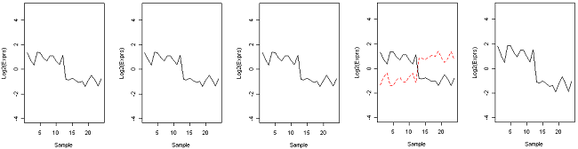
Centered and scaled (z-score = (y - mean) / sd)
It is interesting that the gene expression literature has a fair amount of discussion about what kind of clustering to use, and almost no discussion about what distance method to use. And yet, as you will see in a later example of the two most common methods of clustering, using the same distance measure the clusters look nearly identical. You can very easily see that they have the same expression patterns. The bottom line is, what really matters is the distance measure. Correlation works well for gene expression in clustering both samples and genes.
Pearson's correlation is quite sensitive to outliers. This does not matter when clustering samples, because the correlation is over thousands of genes. When clustering genes, it is important to be aware of the possible impact of outliers. This can be mitigated by using Spearman's correlation instead of Pearson's correlation.
Defining Cluster Distance: The Linkage Function
So far we have defined a distance between items. The linkage function tells you to measure the distance between clusters. Again, there are many choices. Typically you consider either a new item that summarizes the items in the cluster, or a new distance that summarizes the distance between the items in the cluster and items in other clusters. Here is a list of four methods. In each example, x is in one cluster and y is in the other.
name of linkage function form of linkage function
| Single (string-like, long) | \(f = min(d(x,y))\) |
| Complete (ball-like, compact) |
\(f = max(d(x,y))\) |
| Average (ball-like, compact) |
\(f = average(d(x,y))\) |
| Centroid (ball-like, compact) |
\(d(ave(X),ave(Y) )\) where we take the average over all items in each cluster |
For example, suppose we have two clusters \(C_I\) and \(C_2\) with elements \(x_{ij}\) where i is the cluster and j is the item in the cluster. \(D(C_1, C_2)\) is a function of the distances \(f \{d(x_{1j}, x_{2k}) \}\).
Single linkage clusters looks at all the pairwise distances between the items in the two clusters and takes the distance between the clusters as the minimum distance.
Complete linkage, which is more popular, takes the maximum distance.
Average linkage takes the average, which as it turns out is fairly similar to complete linkage.
Centroid linkage sounds the same as average linkage but instead of using the average distance, it creates a new item which is the average of all the individual items and then uses the distance between averages.
Single and complete linkage give the same dendrogram whether you use the raw data, the log of the data or any other transformation of the data that preserves the order because what matters is which ones have the smallest distance. The other methods are sensitive to the measurement scale. The most popular methods for gene expression data are to use log2(expression + 0.25), correlation distance and complete linkage clustering.

