Printer-friendly version

Example of Complete Linkage Clustering

Clustering starts by computing a distance between every pair of units that you want to cluster.  A distance matrix will be symmetric (because the distance between x and y is the same as the distance between y and x) and will have zeroes on the diagonal (because every item is distance zero from itself).  The table below is an example of a distance matrix.  Only the lower triangle is shown, because the upper triangle can be filled in by reflection.

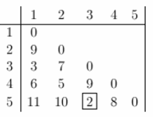
Now lets start clustering.  The smallest distance is between three and five and they get linked up or merged first into a the cluster '35'.

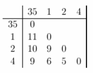
 To obtain the new distance matrix, we need to remove the 3 and 5 entries, and replace it by an entry "35" .  Since we are using complete linkage clustering, the distance between "35" and every other item is the maximum of the distance between this item and 3 and this item and 5.  For example, d(1,3)= 3 and d(1,5)=11.  So, D(1,"35")=11.  This gives us the new distance matrix.  The items with the smallest distance get clustered next.  This will be 2 and 4.

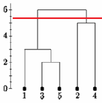
Continuing in this way, after 6 steps, everything is clustered. This is summarized below.  On this plot, the y-axis shows the distance between the objects at the time they were clustered.  This is called the cluster height.  Different visualizations use different measures of cluster height.

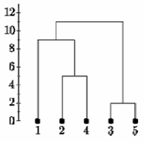
Complete Linkage

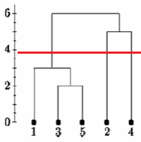
Below is the single linkage dendrogram for the same distance matrix.  It starts with cluster "35" but the distance between "35" and each item is now the minimum of d(x,3) and d(x,5).  So c(1,"35")=3.

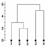
Single Linkage

Determining clusters

One of the problems with hierarchical clustering is that there is no objective way to say how many clusters there are. 

If we cut the single linkage tree at the point shown below, we would say that there are two clusters.

However, if we cut the tree lower we might say that there is one cluster and two singletons.

There is no commonly agreed-upon way to decide where to cut the tree.

Let's look at some real data.  In homework 5 we consider gene expression in 4 regions of 3 human and 3 chimpanzee brains.  The RNA was hybridized to Affymetrix human gene expression microarrays.  We normalized the data using RMA and did a differential expression analysis using LIMMA.  Here we selected the 200 most significantly differentially expressed genes from the study. We cluster all the differentially expressed genes based on their mean expression in each of the 8 species by brain region treatments

Here are the clusters based on Euclidean distance and correlation distance, using complete and single linkage clustering.

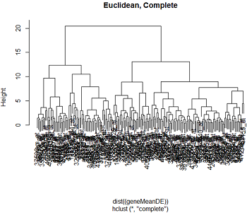
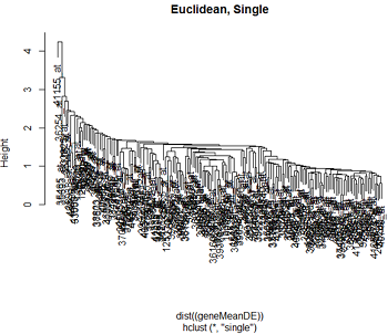
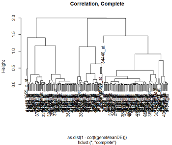
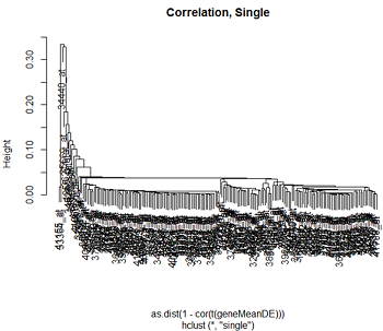
We can see that the clustering pattern for complete linkage distance tends to create compact clusters of clusters, while single linkage tends to add one point at a time to the cluster, creating long stringy clusters.  As we might expect from our discussion of distances, Euclidean distance and correlation distance produce very different dendrograms.  

Hierarchical clustering does not tell us how many clusters there are, or where to cut the dendrogram to form clusters.  In R there is a function cutttree which will cut a tree into clusters at a specified height.  However, based on our visualization, we might prefer to cut the long branches at different heights.  In any case, there is a fair amount of subjectivity in determining which branches should and should not be cut to form separate clusters. 

Understanding the clusters

To understand the clusters we usually plot the log2(expression) values of the genes in the cluster, or in other words, plot the gene expressions over the samples. (The numbering in these graphs are totally arbitrary.)  Even though the treatments are unordered, I usually connect the points coming from a single feature to make the pattern clearer.  These are called profile plots.

Here is some of the profile plots from complete linkage clustering when we used Euclidean distance:

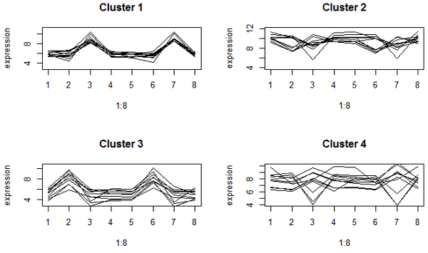
These look very tightly packed.  However, clusters 2 and 4 have genes with different up and down patterns, because they have about the same mean expression.  Cluster 2 are very highly expressed genes.

Here's what we got when we use correlation distance:

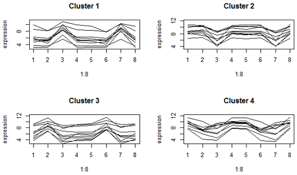
These are much looser on the y-axis because correlation focuses on the expression pattern, not the mean.  However, all the genes in the same cluster have a peak or valley in the same treatments (which are brain regions by species combinations).  Clusters 1 and 2 are genes that are respectively higher or lower in the cerebellum compared to other brain regions in both species. 

Selecting a gene list 

In principle it is possible to cluster all the genes, although visualizing a huge dendrogram might be problematic.  Usually, some type of preliminary analysis, such as differential expression analysis is used to select genes for clustering.  There are good reasons to do so, although there are also some caveats.

Typically in gene expression, the distance metric used is correlation distance.  Correlation distance is the same as centering and scaling the data, and then using Euclidean distance.  When there are systematic treatment effects, we expect the variability of gene expression from treatment to treatment to be a mix of systematic treatment effects and noise.  When there are no treatment effects, the variability of gene expression is just due to noise.  However, centering and scaling the data puts all variabity on the same scale.  Hence genes that exhibit a pattern due to chance are not distinguishable from those that have a systematic component.   

As we have seen, correlation distance has better biological interpretation than Euclidean distance for gene expression studies, but the same scaling that makes it useful for finding biologically meaningful patterns of gene regulation introduces spurious results for genes that do not differentially express.  Selecting genes based on differential expression analysis removes genes which are likely to have only chance patterns.  This should enhance the patterns found in the gene clusters.

As a caveat, however, consider the effects of gene selection on clustering samples or treatments.  The selected genes are those which test positive in differential expression analysis.  Use of those genes to cluster samples is biased towards clustering the samples by treatment.