Printer-friendly version

K means or K mediods clustering are other popular methods for clustering.  They require as input the data, the number K of clusters you expect, and K "centers" which are used to start the algorithm.  The centers have the same format as one of the data vectors.  As the algorithm progresses, the centers are recomputed along with the clusters.

The algorithm proceeds by assigning each data value to the nearest center.  This creates K clusters.  Then a new cluster center is selected based on the data in the cluster.  For the K-means algorithm, the distance is always Euclidean distance and the new center is the component-wise mean of the data in the cluster.  To use correlation distance, the data are input as z-scores.  For the K-mediods algorithm, other distances can be used and the new center is one of the data values in the cluster.  

If there are no well-separated clusters in the data (the usual case) then the clusters found by the algorithm may depend on the starting values.  For this reason, it is common to try the algorithm with different starting values.

The K-means method is sensitive to anomalous data points and outliers. If you have an outlier then whatever cluster it would be included in, the centroid of that cluster would be pulled out to towards that point. The K-mediod method is robust to outliers when robust distance measures such as Manhattan distance are used. 

At each step of the algorithm, all the points may be reassigned to new clusters.  This means that mistaken cluster assignments early in the process are corrected later on.

If two centers are equally (and maximally) close to an observation at a given iteration, we have to choose arbitrarily which one to cluster it with. The problem here is not as serious as in hierarchical clustering because points can move in later iterations.

The algorithm minimizes the total within cluster distance. This is basically like the average distance between the center of a cluster and everything in the cluster.  Clusters tend to be ball shaped with respect to the chosen distance.

Here is a case that is pretty ideal because you have to clearly separated clusters. Suppose we started at the open rectangles.

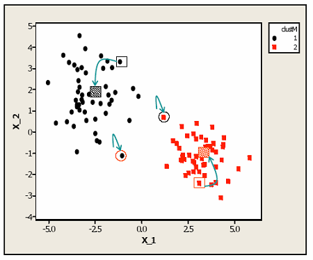
The points that are closest to one of the open rectangles get put into a cluster defined by the centroid. All the points nearest each of the open rectangles is shown in color here.  The centroids were then recomputed based on this current clustering leading to the centroids being recomputed as the dashed rectangles. Data values are then reassigned to clusters and the process is repeated. In this example, only the two points with circles around them are assigned to new clusters in the second step.  The process is repeated until the clusters (and hence the cluster centroids) do not change.

The algorithm doesn't tell you how to pick the number of clusters. There are some measures about how tight the clusters are that could be used for this however.

Two-dimensional sets of points are easier to visualize than, for instance, our example with eight dimensions defined by the treatment means and 200 genes. This makes it much more difficult to see the clusters visually.  However, it turns out that K-means clustering is closely associated mathematically with a method called principal components analysis (PCA).  PCA picks out directions of maximal variance from high dimensional data (e.g. for gene expression, the expression value in one treatment is a dimension; for clustering samples, the expression of each gene in the sample is a dimension).  Scatterplots using the first 2 or 3 principal components can often be used to visualize the data in a way that clearly shows the clusters from K-means.  K-mediods is not mathematically associated with PCA, but the first 2 or 3 principal components still often do a good job of displaying the clusters.

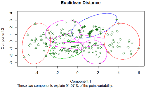
Below we show the PCA visualization of the brain data with 8 treatment means of the 200 most differentially express genes.    We used k-mediod clustering with K=6 clusters and Euclidean distance.  Where clusters overlap on the plot, they might actually be separated if we could display 3 dimensions.  However, even in 2 dimensions we see that the clusters are quite well separated.

Using correlation distance for the brain data we obtain:

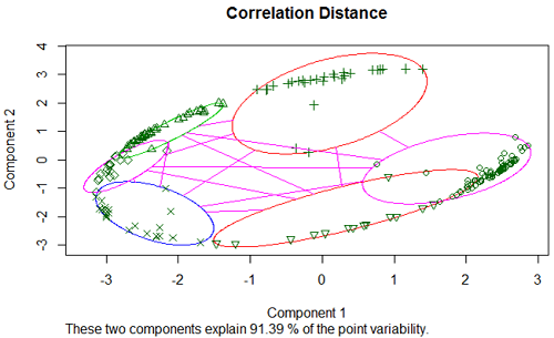
Because correlations are squeezed between -1 and 1, the principal components plot of the correlation distance often has this elliptical shape, with most of the data on the boundary of the ellipse.  The clusters are still clearly separated.

However, the plots also show another problem with clustering with selected genes.  In a certain sense we can see that the separation into clusters is arbitrary - we could rotate the elliptical cluster boundaries around the boundary of the main ellipse, and we would still see clustered structure.  What we are doing is what Bryan [1] called 'zip coding'. This is an arbitrary way of putting nearby units into clusters with arbitrary boundaries just as zip-codes are arbitrary geographical boundaries.

Clustering is an exploratory method that helps us visualize the data but it is only ruseful if it matches up with something biological that we can interpret. Before data mining became a standard part of machine learning, statisticians used to talk about data mining as a form of p-hacking,  looking for patterns that may or may not be real. Clustering is very much in this 'searching for significance' mind-set. If the resulting clusters up with something interpretable, this is good, but you still have to validate the clustering by taking another sample or using someone else's data to to see if you get the same patterns.

We can also look at the cluster contents by looking at the profiles. These graphs using both  K-mediods  (top) and complete linkage clustering (bottom) look very much the same here.  Both methods try to find "spherical" clusters, and the cluster patterns look very similar.  This gives us greater confidence that the clusters have picked out some meaningful patterns in our data.

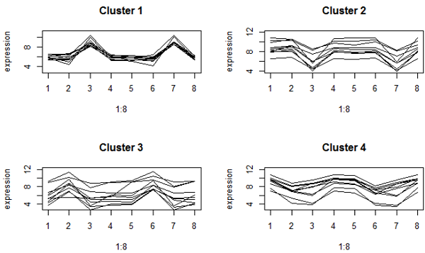
K-mediods method

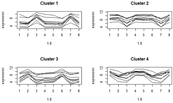
Complete linkage hierarchical clustering