11.11 - Bagging
There is a very powerful idea in the use of subsamples of the data and in averaging over subsamples through bootstrapping.
Bagging exploits that idea to address the overfitting issue in a more fundamental manner. It was invented by Leo Breiman, who called it "bootstrap aggregating" or simply "bagging" (see the reference: "Bagging predictors," Machine Learning, 24:123-140, 1996, cited by 7466).
In a classification tree, bagging takes a majority vote from classifiers trained on bootstrap samples of the training data.
Algorithm: Consider the following steps in a fitting algorithm with a dataset having N observations and a binary response variable.
-
Take a random sample of size N with replacement from the data (a bootstrap sample).
-
Construct a classification tree as usual but do not prune.
-
Assign a class to each terminal node, and store the class attached to each case coupled with the predictor values for each observation.
-
Repeat Steps 1-3 a large number of times.
-
For each observation in the dataset, count the number of trees that it is classified in one category over the number of trees.
-
Assign each observation to a final category by a majority vote over the set of trees. Thus, if 51\% of the time over a large number of trees a given observation is classified as a "1'', that becomes its classification.
Although there remain some important variations and details to consider, these are the key steps to producing "bagged'' classification trees. The idea of classifying by averaging over the results from a large number of bootstrap samples generalizes easily to a wide variety of classifiers beyond classification trees.
Margins:
Bagging introduces a new concept, "margins." Operationally, the "margin" is the difference between the proportion of times a case is correctly classified and the proportion of times it is incorrectly classified. For example, if over all trees an observation is correctly classified 75\% of the time, the margin is 0.75 - 0.25 = 0.50.
Large margins are desirable because a more stable classification is implied. Ideally, there should be large margins for all of the observations. This bodes well for generalization to new data.
Out-Of-Bag Observations:
For each tree, observations not included in the bootstrap sample are called "out-of-bag'' observations. These "out-of-bag'' observations can be treated as a test dataset, and dropped down the tree.
To get a better evaluation of the model, the prediction error is estimated only based on the "out-of-bag'' observations. In other words, the averaging for a given observation is done only using the trees for which that observation was not used in the fitting process.
Example: Domestic Violence
Why Bagging Works? The core of bagging's potential is found in the averaging over results from a substantial number of bootstrap samples. As a first approximation, the averaging helps to cancel out the impact of random variation. However, there is more to the story, some details of which are especially useful for understanding a number of topics we will discuss later.
Data were collected to help forecast incidents of domestic violence within households. For a sample of households to which sheriff's deputies were dispatched for domestic violence incidents, the deputies collected information on a series of possible predictors of future domestic violence, for example, whether police officers had been called to that household in the recent past.
The following three figures are three classification trees constructed from the same data, but each using a different bootstrap sample.
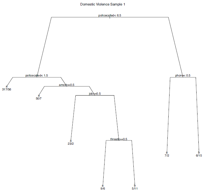
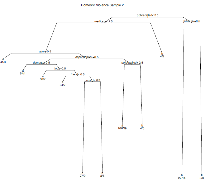
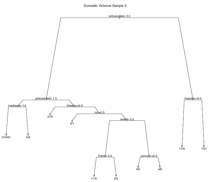
It is clear that the three figures are very different. Unstable results may be due to any number of common problems: small sample sizes, highly correlated predictors; or heterogeneous terminal nodes. Interpretations from the results of a single tree can be quite risky when a classification tree performs in this manner. However, when a classification tree is used solely as a classification tool, the classes assigned may be relatively stable even if the tree structure is not.
The same phenomenon can be found in conventional regression when predictors are highly correlated. The regression coefficients estimated for particular predictors may be very unstable, but it does not necessarily follow that the fitted values will be unstable as well.
It is not clear how much bias exists in the three trees. But it is clear that the variance across trees is large. Bagging can help with the variance. The conceptual advantage of bagging is to aggregate fitted values from a large number of bootstrap samples. Ideally, many sets of fitted values, each with low bias but high variance, may be averaged in a manner than can effectively reduce the bite of the bias-variance tradeoff. The ways in which bagging aggregates the fitted values is the basis for many other statistical learning developments.
Bagging a Quantitative Response:
Recall that a regression tree maximizes the reduction in the error sum of squares at each split. All of the concerns about overfitting apply, especially given the potential impact that outliers can have on the fitting process when the response variable is quantitative. Bagging works by the same general principles when the response variable is numerical.
- For each tree, each observation is placed in a terminal node and assigned the mean of that terminal node.
- Then, the average of these assigned means over trees is computed for each observation.
- This average value for each observation is the bagged fitted value.
R Package for Bagging:
In R, the bagging procedure (i.e., bagging() in the ipred library) can be applied to classification, regression, and survival trees.
"nbagg'' gives an integer giving the number of bootstrap replications. "control'' gives control details of the rpart algorithm.
We can also use the random forest procedure in the "randomForest" package since bagging is a special case of random forests.

