Printer-friendly version

Here we have 10 digits, 0 through 9, and as you might see on a calculator, they are displayed by different on-off combinations of seven horizontal and vertical light bars.

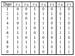
In this case, each digit is represented by a 7-dimensional vector of zeros and ones. The ith sample is \(x_i = (x_{i1} , x_{i2}, \cdots , x_{i7})\). If \(x_{ij} = 1\), the jth light is on; if \(x_{ij} = 0\), the jth light is off.

If the calculator works properly, the following table shows which light bars should be turned on or off for each of the digit.

Let's suppose that the calculator is malfunctioning. Each of the seven lights has probability 0.1 of being in the wrong state independently. In the training data set 200 samples are generated according to the specified distribution.

A classification tree is applied to this dataset. For this data set, each of the seven variables takes only two possible values: 0 and 1. Therefore, for every variable, the only possible candidate question is whether the value is on (1) or off (0). Consequently, we only have seven questions in the candidate pool: Is \(x_{. j}= 0?, j = 1, 2, \cdots , 7\).

In this example the twoing rule is used in splitting instead of the goodness of split based on an impurity function. Also, the result presented was obtained using pruning and cross-validation.

Classification Performance - Results:

• The error rate estimated by using an independent test dataset of size 5000 is 0.30.
• The error rate estimated by cross-validation using the training dataset which only contains 200 data points is also 0.30. In this case, the cross validation did a very good job for estimating the error rate.
• The resubstitution estimate of the error rate is 0.29. This is slightly more optimistic than the true error rate.

Here pruning and cross validation effectively help avoid over fitting. If we don't prune and grow the tree too big, we might get a very small resubstitution error rate which is substantially smaller than the error rate based on the test data set.

• The Bayes error rate is 0.26. Remember, we know the exact distribution for generating the simulated data.  Therefore the Bayes rule using the true model is known.
• There is little room for improvement over the tree classifier.

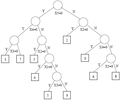
The tree obtained is shown below:

We can see that the first question checks the on/off status of the fifth light. We ask whether \(x_5 = 0\). If the answer is yes (the light is off), go to the left branch. If the answer is no, take the right branch. For the left branch, we ask whether the fourth light, \(x_4\), is on or off. If the answer is yes, then we check the first light, \(x_1\). If \(x_1\) is off then we say that it is digit 1, if the answer is no then it is a 7. The square nodes are leaf nodes, and the number in the square is the class label, or the digit, assigned to the leaf node.

In general, one class may occupy several leaf nodes and occasionally no leaf node.

Interestingly, in this example, every digit (or every class) occupies exactly one leaf node. There are exactly 10 leaf nodes. But this is just a special case.

Another interesting aspect about the tree in this example is that x₆ and x₇ are never used. This shows that classification trees sometimes achieve dimension reduction as a by-product.

Example: Waveforms

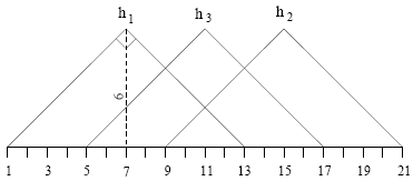
Let's take a look at another example concerning wave forms. Let's first define three functions \(h_1(\tau), h_2(\tau), h_3(\tau)\) which are shifted versions of each other, as shown in the figure below:

We specify each \(h_j\) by its values at integers \(\tau =1 \tilde 21\). Therefore, every wave form is characterized by a 21 dimensional vector.

Next, we will create in the following manner three classes of waveforms as random convex combinations of two of these waveforms plus independent Gaussian noise. Each sample is a 21 dimensional vector containing the values of the random waveforms measured at \(\tau = 1, 2, \cdots , 21\).

To generate a sample in class 1, first we generate a random number υ uniformly distributed in [0, 1] and then we generate 21 independent random numbers \(\epsilon_1, \epsilon_2, \cdots , \epsilon_{21}\) normally distributed with mean = 0 and variance 1 (they are Gaussian noise.) Now, we can create a random waveform by a random sum of \(h_1(j)\) and \(h_2(j)\) with the weights given by the random number picked from the interval [0, 1]:

\[x_{·j} = uh_1(j) + (1 - \nu) h_2(j) + \epsilon_j,  \;\;\;\;    j = 1, \cdots , 21\]

This is a convex combination where the weights are nonnegative and add up to one, with Gaussian noise, \(\epsilon_j\), added on top.

Similarly, to generate a sample in class 2, we repeat the above process to generate a random number \(\nu\) and 21 random numbers \(\epsilon_1, \cdots , \epsilon_{21}\) and set

\[x_{·j} = uh_1(j) + (1 - \nu) h_3(j) + \epsilon_j,   \;\;\;\;    j = 1, \cdots , 21\]

This is a convex combination of \(h_1(j)\) and \(h_3(j)\) plus noise.

Then, the class 3 vectors are generated by a convex combination of \(h_2(j)\) and \(h_3(j)\) plus noise:

\[x_{·j} = uh_2(j) + (1 - \nu) h_3(j) + \epsilon_j,  \;\;\;\;     j = 1, \cdots , 21\]

Below are sample random waveforms generated according to the above description.

Let's see how a classification tree performs.

Here we have generated 300 random samples using prior probabilities (1/3, 1/3, 1/3) for training.

The set of splitting questions are whether x_j is smaller than or equal to a threshold c:

{Is \(x_{·j} \leq c?\)} for c ranging over all real numbers and j = 1, ... , 21

Next, we use the Gini index as the impurity function and compute the goodness of split correspondingly.

Then the final tree is selected by pruning and cross-validation.

Results:

• The cross-validation estimate of misclassification rate is 0.29.
• The misclassification rate on a separate test dataset of size 5000 is 0.28.
  • This is pretty close to the cross-validation estimate!
• The Bayes classification rule can be derived because we know the underlying distribution of the three classes. Applying this rule to the test set yields a misclassification rate of 0.14.

We can see that in this example, the classification tree performs much worse than the theoretical optimal classifier.

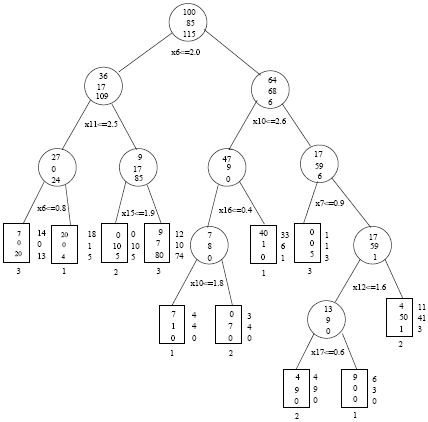
Here is the tree. Again, the corresponding question used for every split is placed below the node. Three numbers are put in every node, which indicate the number of points in every class for that node. For instance in the root node at the top, there are 100 points in class 1, 85 points in class 2, and 115 in class 3. Although the prior probabilities used were all one third, because random sampling is used, there is no guarantee that in the real data set the numbers of points for the three classes are identical.

If we take a look at the internal node to the left of the root node, we see that there are 36 points in class 1, 17 points in class 2 and 109 points in class 3, the dominant class. If we look at the leaf nodes represented by the rectangles, for instance the leaf node on the far left, it has seven points in class 1, 0 points in class 2 and 20 points in class 3. According to the class assignment rule, we would choose a class that dominates this leaf node, 3 in this case. Therefore, this leaf node is assigned to class 3, shown by the number below the rectangle. In the leaf node to its right, class 1 with 20 data points is most dominant, and hence assigned to this leaf node.

We also see numbers on the right of the rectangles representing leaf nodes. These numbers indicate how many test data points in each class land in the corresponding leaf node. For the ease of comparison with the numbers inside the rectangles, which are based on the training data, the numbers based on test data are scaled to have the same sum as that on training.

Also, observe that although we have 21 dimensions, many of these are not used by the classification tree. The tree is relatively small.