Printer-friendly version

Under LDA we assume that the density for X, given every class k is following a Gaussian distribution. Here is the density formula for a multivariate Gaussian distribution:

\[f_k(x)=\dfrac{1}{(2\pi)^{p/2}|\Sigma_k|^{1/2}} e^{-\frac{1}{2}(x-\mu_k)^T\Sigma_{k}^{-1}(x-\mu_k)}\]

p is the dimension and \(\Sigma_k\) is the covariance matrix. This involves the square root of the determinant of this matrix. In this case, we are doing matrix multiplication. The vector x and the mean vector \(\mu_k\) are both column vectors.

For Linear discriminant analysis (LDA): \(\Sigma_k=\Sigma\), ∀k.

In LDA, as we mentioned, you simply assume for different k that the covariance matrix is identical. By making this assumption, the classifier becomes linear. The only difference from quadratic discriminant analysis is that we do not assume that the covariance matrix is identical for different classes. For QDA, the decision boundary is determined by a quadratic function.

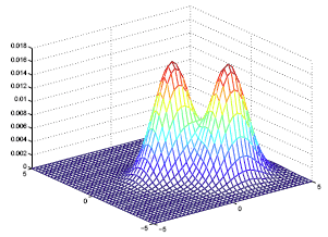
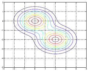
Since the covariance matrix determines the shape of the Gaussian density, in LDA, the Gaussian densities for different classes have the same shape, but are shifted versions of each other (different mean vectors).  Example densities for the LDA model are shown below.