Printer-friendly version

QDA is not really that much different from LDA except that you assume that the covariance matrix can be different for each class and so, we will estimate the covariance matrix \(\Sigma_k\) separately for each class k, k =1, 2, ... , K.

Quadratic discriminant function:

\[\delta_k(x)= -\frac{1}{2}\text{log}|\Sigma_k|-\frac{1}{2}(x-\mu_{k})^{T}\Sigma_{k}^{-1}(x-\mu_{k})+\text{log}\pi_k\]

This quadratic discriminant function is very much like the linear discriminant function except that because Σ_k, the covariance matrix, is not identical, you cannot throw away the quadratic terms. This discriminant function is a quadratic function and will contain second order terms.

Classification rule:

\[\hat{G}(x)=\text{arg }\underset{k}{\text{max }}\delta_k(x)\]

The classification rule is similar as well. You just find the class k which maximizes the quadratic discriminant function.

The decision boundaries are quadratic equations in x.

QDA, because it allows for more flexibility for the covariance matrix, tends to fit the data better than LDA, but then it has more parameters to estimate. The number of parameters increases significantly with QDA. Because, with QDA, you will have a separate covariance matrix for every class. If you have many classes and not so many sample points, this can be a problem.

As we talked about at the beginning of this course, there are trade-offs between fitting the training data well and having a simple model to work with. A simple model sometimes fits the data just as well as a complicated model. Even if the simple model doesn't fit the training data as well as a complex model, it still might be better on the test data because it is more robust.

QDA Example - Diabetes Data Set

In this example we do the same things as we have previously with LDA on the prior probabilities and the mean vectors, except now we estimate the covariance matrices separately for each class.

How do we estimate the covariance matrices separately?

Remember, in LDA once we had the summation over the data points in every class we had to pull all the classes together. In QDA we don't do this.

Prior probabilities: \(\hat{\pi}_0=0.651, \hat{\pi}_1=0.349  \). 

\(\hat{\mu}_0=(-0.4038, -0.1937)^T, \hat{\mu}_1=(0.7533, 0.3613)^T  \)

\(\hat{\Sigma_0}= \begin{pmatrix}
 1.6790 & -0.0461 \\
-0.0461 & 1.5985
\end{pmatrix}  \)

\(\hat{\Sigma_1}= \begin{pmatrix}
 2.0114 & -0.3334 \\
-0.3334 & 1.7910
\end{pmatrix}  \)

The dashed line in the plot below is decision boundary given by LDA.The curved line is the decision boundary resulting from the QDA method.

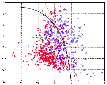
For most of the data, it doesn't make any difference, because most of the data is massed on the left. The percentage of the data in the area where the two decision boundaries differ a lot is small.  Therefore, you can imagine that the difference in the error rate is very small.

• Within training data classification error rate: 29.04%.
• Sensitivity: 45.90%.
• Specificity: 84.40%.

Sensitivity for QDA is the same as that obtained by LDA, but specificity is slightly lower.