Printer-friendly version

LDA makes some strong assumptions. It assumes that the covariance matrix is identical for different classes. It also assumes that the density is Gaussian. What if these are not true?  LDA may not necessarily be bad when the assumptions about the density functions are violated. Here are some examples that might illustrate this.

In certain cases, LDA may yield poor results.

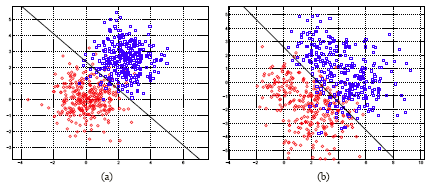
In the first example (a), we do have similar data sets which follow exactly the model assumptions of LDA. This means that the two classes, red and blue, actually have the same covariance matrix and they are generated by Gaussian distributions. Below, in the plots, the black line represents the decision boundary. The second example (b) violates all of the assumptions made by LDA. First of all the within class of density is not a single Gaussian distribution, instead it is a mixture of two Gaussian distributions. The overall density would be a mixture of four Gaussian distributions. Also, they have different covariance matrices as well.

Then, if we apply LDA we get this decision boundary (above, black line), which is actually very close to the ideal boundary between the two classes. By ideal boundary, we mean the boundary given by the Bayes rule using the true distribution (since we know it in this simulated example).

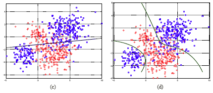
If you look at another example, (c) below, here we also generated two classes. The red class still contains two Gaussian distributions. The blue class, which spreads itself over the red class with one mass of data in the upper right and another data mass in the lower left. If we force LDA we get a decision boundary, as displayed. In this case the result is very bad (far below ideal classification accuracy). You can see that in the upper right the red and blue are very well mixed, however, in the lower left the mix is not as great.  You can imagine that the error rate would be very high for classification using this decision boundary.

In plot (d), the density of each class is estimated by a mixture of two Gaussians.  The Bayes rule is applied.  The resulting boundaries are two curves.   The separation of the red and the blue is much improved.

This example illustrates when LDA gets into trouble. LDA separates the two classes with a hyper plane. This means that the two classes have to pretty much be two separated masses, each occupying half of the space.  In the above example,  the blue class breaks into two pieces, left and right. Then, you have to use more sophisticated density estimation for the two classes if you want to get a good result. This is an example where LDA has seriously broken down. This is why it's always a good idea to look at the scatter plot before you choose a method. The scatter plot will often show whether a certain method is appropriate. If you see a scatter plot like this example, you can see that the blue class is broken into pieces, and you can imagine if you used LDA, no matter how you position your linear boundary, you are not going to get a good separation between the red and the blue class. Largely you will find out that LDA is not appropriate and you want to take another approach.