In this lesson, we’ll describe some important features that we must consider when describing and modeling a time series. This is meant to be an introductory overview, illustrated by example, and not a complete look at how we model a univariate time series. Here, we’ll only consider univariate time series. We’ll examine relationships between two or more time series later on.
- Univariate Time Series
- A univariate time series is a sequence of measurements of the same variable collected over time. Most often, the measurements are made at regular time intervals.
One difference from standard linear regression is that the data are not necessarily independent and not necessarily identically distributed. One defining characteristic of a time series is that it is a list of observations where the ordering matters. Ordering is very important because there is dependency and changing the order could change the meaning of the data.
Basic Objectives of the Analysis
The basic objective usually is to determine a model that describes the pattern of the time series. Uses for such a model are:
- To describe the important features of the time series pattern.
- To explain how the past affects the future or how two time series can “interact”.
- To forecast future values of the series.
- To possibly serve as a control standard for a variable that measures the quality of product in some manufacturing situations.
Types of Models
There are two basic types of “time domain” models.
- Models that relate the present value of a series to past values and past prediction errors - these are called ARIMA models (for Autoregressive Integrated Moving Average). We’ll spend substantial time on these.
- Ordinary regression models that use time indices as x-variables. These can be helpful for an initial description of the data and form the basis of several simple forecasting methods.
Important Characteristics to Consider First
Some important questions to first consider when first looking at a time series are:
- Is there a trend, meaning that, on average, the measurements tend to increase (or decrease) over time?
- Is there seasonality, meaning that there is a regularly repeating pattern of highs and lows related to calendar time such as seasons, quarters, months, days of the week, and so on?
- Are there outliers? In regression, outliers are far away from your line. With time series data, your outliers are far away from your other data.
- Is there a long-run cycle or period unrelated to seasonality factors?
- Is there constant variance over time, or is the variance non-constant?
- Are there any abrupt changes to either the level of the series or the variance?
Example 1-1 Section
The following plot is a time series plot of the annual number of earthquakes in the world with seismic magnitude over 7.0, for 99 consecutive years. By a time series plot, we simply mean that the variable is plotted against time.
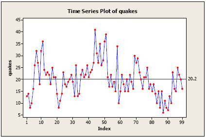
Some features of the plot:
- There is no consistent trend (upward or downward) over the entire time span. The series appears to slowly wander up and down. The horizontal line drawn at quakes = 20.2 indicates the mean of the series. Notice that the series tends to stay on the same side of the mean (above or below) for a while and then wanders to the other side.
- Almost by definition, there is no seasonality as the data are annual data.
- There are no obvious outliers.
- It’s difficult to judge whether the variance is constant or not.
One of the simplest ARIMA type models is a model in which we use a linear model to predict the value at the present time using the value at the previous time. This is called an AR(1) model, standing for autoregressive model of order 1. The order of the model indicates how many previous times we use to predict the present time.
A start in evaluating whether an AR(1) might work is to plot values of the series against lag 1 values of the series. Let \(x_t\) denote the value of the series at any particular time \(t\), so \(x_{t-1}\) denotes the value of the series one time before time \(t\). That is, \(x_{t-1}\) is the lag 1 value of \(x_t\). As a short example, here are the first five values in the earthquake series along with their lag 1 values:
| t | \(x_t\) | \(x_{t-1}\) (lag 1 value) |
|---|---|---|
| 1 | 13 | * |
| 2 | 14 | 13 |
| 3 | 8 | 14 |
| 4 | 10 | 8 |
| 5 | 16 | 10 |
For the complete earthquake dataset, here’s a plot of \(x_t\) versus \(x_{t-1}\) :
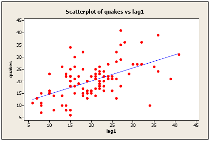
Although it’s only a moderately strong relationship, there is a positive linear association so an AR(1) model might be a useful model.
The AR(1) model
Theoretically, the AR(1) model is written
\(x_t = \delta + \phi_1 x_{t-1} + w_t\)
Assumptions:
- \(w_t \overset{iid}{\sim} N(0, \sigma^2_w)\), meaning that the errors are independently distributed with a normal distribution that has mean 0 and constant variance.
- Properties of the errors \(w_t\) are independent of \(x\).
This is essentially the ordinary simple linear regression equation, but there is one difference. Although it’s not usually true, in ordinary least squares regression we assume that the x-variable is not random but instead is something we can control. That’s not the case here, but in our first encounter with time series we’ll overlook that and use ordinary regression methods. We’ll do things the “right” way later in the course.
Following is Minitab output for the AR(1) regression in this example:
quakes = 9.19 + 0.543 lag1
98 cases used, 1 cases contain missing values
| Predictor | Coef | SE Coef | T | P |
|---|---|---|---|---|
| Constant | 9.191 | 1.819 | 5.05 | 0.000 |
| lag1 | 0.54339 | 0.08528 | 6.37 | 0.000 |
S = 6.12239 R-Sq = 29.7% R-Sq(adj) = 29.0%
We see that the slope coefficient is significantly different from 0, so the lag 1 variable is a helpful predictor. The \(R^2\) value is relatively weak at 29.7%, though, so the model won’t give us great predictions.
Residual Analysis
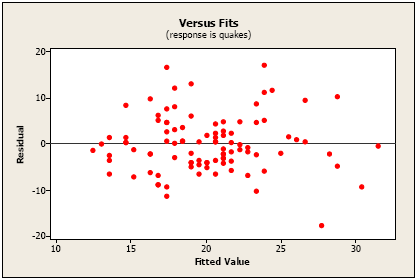
In traditional regression, a plot of residuals versus fits is a useful diagnostic tool. The ideal for this plot is a horizontal band of points. Following is a plot of residuals versus predicted values for our estimated model. It doesn’t show any serious problems. There might be one possible outlier at a fitted value of about 28.
Example 1-2 Section
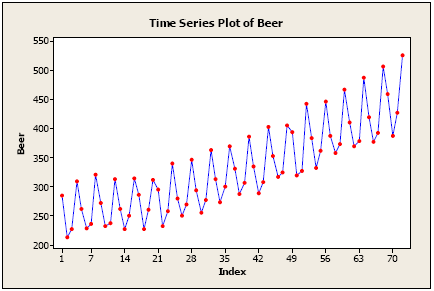
1The following plot shows a time series of quarterly production of beer in Australia for 18 years.
Some important features are:
- There is an upward trend, possibly a curved one.
- There is seasonality – a regularly repeating pattern of highs and lows related to quarters of the year.
- There are no obvious outliers.
- There might be increasing variation as we move across time, although that’s uncertain.
There are ARIMA methods for dealing with series that exhibit both trend and seasonality, but for this example, we’ll use ordinary regression methods.
Classical regression methods for trend and seasonal effects
To use traditional regression methods, we might model the pattern in the beer production data as a combination of the trend over time and quarterly effect variables.
Suppose that the observed series is \(x_t\), for \(t = 1,2, \dots, n\).
- For a linear trend, use \(t\) (the time index) as a predictor variable in a regression.
- For a quadratic trend, we might consider using both \(t\) and \(t^2\).
- For quarterly data, with possible seasonal (quarterly) effects, we can define indicator variables such as \(S_j=1\) if the observation is in quarter \(j\) of a year and 0 otherwise. There are 4 such indicators.
Let \(\epsilon_t \overset{iid}{\sim} N(0, \sigma^2)\). A model with additive components for linear trend and seasonal (quarterly) effects might be written
\(x_t = \beta_1t+\alpha_1S_1+\alpha_2S_2 + \alpha_3S_3 +\alpha_4S_4 + \epsilon_t\)
To add a quadratic trend, which may be the case in our example, the model is
\(x_t = \beta_1t + \beta_2t^2 +\alpha_1S_1 + \alpha_2S_2 + \alpha_3S_3 +\alpha_4S_4 + \epsilon_t\)
We’ve deleted the “intercept” from the model. This isn’t necessary, but if we include it we’ll have to drop one of the seasonal effect variables from the model to avoid collinearity issues.
Back to Example 2: Following is the Minitab output for a model with a quadratic trend and seasonal effects. All factors are statistically significant.
| Predictor | Coef | SE Coef | T | P |
|---|---|---|---|---|
| Noconstant | ||||
| Time | 0.5881 | 0.2193 | 2.68 | 0.009 |
| tsqrd | 0.031214 | 0.002911 | 10.72 | 0.000 |
| quarter_1 | 261.930 | 3.937 | 66.52 | 0.000 |
| quarter_2 | 212.165 | 3.968 | 53.48 | 0.000 |
| quarter_3 | 228.415 | 3.994 | 57.18 | 0.000 |
| quarter_4 | 310.880 | 4.018 | 77.37 | 0.000 |
Residual Analysis
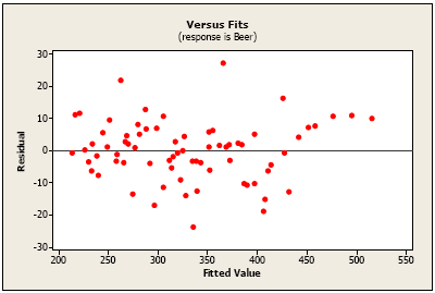
For this example, the plot of residuals versus fits doesn’t look too bad, although we might be concerned by the string of positive residuals at the far right.
When data are gathered over time, we typically are concerned with whether a value at the present time can be predicted from values at past times. We saw this in the earthquake data of example 1 when we used an AR(1) structure to model the data. For residuals, however, the desirable result is that the correlation is 0 between residuals separated by any given time span. In other words, residuals should be unrelated to each other.
Sample Autocorrelation Function (ACF) Section
The sample autocorrelation function (ACF) for a series gives correlations between the series \(x_t\) and lagged values of the series for lags of 1, 2, 3, and so on. The lagged values can be written as \(x_{t-1}, x_{t-2}, x_{t-3}\), and so on. The ACF gives correlations between \(x_t\) and \(x_{t-1}\), \(x_t\) and \(x_{t-2}\), and so on.
The ACF can be used to identify the possible structure of time series data. That can be tricky going as there often isn’t a single clear-cut interpretation of a sample autocorrelation function. We’ll get started on that in Lesson 1.2 this week. The ACF of the residuals for a model is also useful. The ideal for a sample ACF of residuals is that there aren’t any significant correlations for any lag.
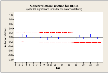
Following is the ACF of the residuals for Example 1, the earthquake example, where we used an AR(1) model. The "lag" (time span between observations) is shown along the horizontal, and the autocorrelation is on the vertical. The red lines indicated bounds for statistical significance. This is a good ACF for residuals. Nothing is significant; that’s what we want for residuals.
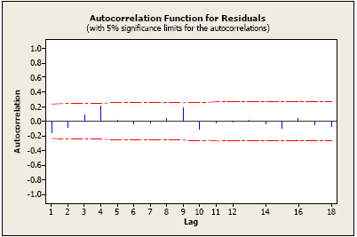
The ACF of the residuals for the quadratic trend plus seasonality model we used for Example 2 looks good too. Again, there appears to be no significant autocorrelation in the residuals. The ACF of the residual follows:
Lesson 1.2 will give more details about the ACF. Lesson 1.3 will give some R code for examples in Lesson 1.1 and Lesson 1.2.