Seasonality in a time series is a regular pattern of changes that repeats over S time periods, where S defines the number of time periods until the pattern repeats again.
For example, there is seasonality in monthly data for which high values tend always to occur in some particular months and low values tend always to occur in other particular months. In this case, S = 12 (months per year) is the span of the periodic seasonal behavior. For quarterly data, S = 4 time periods per year.
In a seasonal ARIMA model, seasonal AR and MA terms predict \(x_{t}\) using data values and errors at times with lags that are multiples of S (the span of the seasonality).
- With monthly data (and S = 12), a seasonal first order autoregressive model would use \(x_{t-12}\) to predict \(x_{t}\). For instance, if we were selling cooling fans we might predict this August’s sales using last August’s sales. (This relationship of predicting using last year’s data would hold for any month of the year.)
- A seasonal second order autoregressive model would use \(x_{t-12}\) and \(x_{t-24}\) to predict \(x_{t}\). Here we would predict this August’s values from the past two Augusts.
- A seasonal first order MA(1) model (with S = 12) would use \(w_{t-12}\) as a predictor. A seasonal second order MA(2) model would use \(w_{t-12}\) and \(w_{t-24}\)
Differencing
Almost by definition, it may be necessary to examine differenced data when we have seasonality. Seasonality usually causes the series to be nonstationary because the average values at some particular times within the seasonal span (months, for example) may be different than the average values at other times. For instance, our sales of cooling fans will always be higher in the summer months.
- Seasonal differencing
-
Seasonal differencing is defined as a difference between a value and a value with lag that is a multiple of S.
- With S = 12, which may occur with monthly data, a seasonal difference is \(\left( 1 - B ^ { 12 } \right) x _ { t } = x _ { t } - x _ { t - 12 }\).
The differences (from the previous year) may be about the same for each month of the year giving us a stationary series.
- With S = 4, which may occur with quarterly data, a seasonal difference is \(\left( 1 - B ^ { 4 } \right) x _ { t } = x _ { t } - x _ { t - 4 }\).
Seasonal differencing removes seasonal trend and can also get rid of a seasonal random walk type of nonstationarity.
- Non-seasonal differencing
-
If trend is present in the data, we may also need non-seasonal differencing. Often (not always) a first difference (non-seasonal) will “detrend” the data. That is, we use \(( 1 - B ) x _ { t } = x _ { t } - x _ { t - 1 }\) in the presence of trend.
- Differencing for Trend and Seasonality
-
When both trend and seasonality are present, we may need to apply both a non-seasonal first difference and a seasonal difference.
That is, we may need to examine the ACF and PACF of \(\left( 1 - B ^ { 12 } \right) ( 1 - B ) x _ { t } = \left( x _ { t } - x _ { t - 1 } \right) - \left( x _ { t - 12 } - x _ { t - 13 } \right)\).
Removing trend doesn't mean that we have removed the dependency. We may have removed the mean, \(\mu_t\), part of which may include a periodic component. In some ways we are breaking the dependency down into recent things that have happened and long-range things that have happened.
Non-seasonal behavior will still matter...
With seasonal data, it is likely that short run non-seasonal components will still contribute to the model. In the monthly sales of cooling fans mentioned above, for instance, sales in the previous month or two, along with the sales from the same month a year ago, may help predict this month’s sales.
We’ll have to look at the ACF and PACF behavior over the first few lags (less than S) to assess what non-seasonal terms might work in the model.
Seasonal ARIMA Model
The seasonal ARIMA model incorporates both non-seasonal and seasonal factors in a multiplicative model. One shorthand notation for the model is
ARIMA \((p, d, q) \times (P, D, Q)S\)
with p = non-seasonal AR order, d = non-seasonal differencing, q = non-seasonal MA order, P = seasonal AR order, D = seasonal differencing, Q = seasonal MA order, and S = time span of repeating seasonal pattern.
Without differencing operations, the model could be written more formally as
(1) \(\Phi(B^S)\phi(B)(x_t-\mu)=\Theta(B^S)\theta(B)w_t\)
The non-seasonal components are:
- AR: \(\phi(B)=1-\phi_1B-\ldots-\phi_pB^p \)
- MA: \(\theta(B) = 1+ \theta_1B+ \ldots + \theta_qB^q \)
The seasonal components are:
- Seasonal AR: \(\Phi(B^S) = 1- \Phi_1 B^S - \ldots - \Phi_PB^{PS} \)
- Seasonal MA: \(\Theta(B^S) = 1 + \Theta_1 B^S + \ldots + \Theta_Q B^{QS} \)
On the left side of equation (1) the seasonal and non-seasonal AR components multiply each other, and on the right side of equation (1) the seasonal and non-seasonal MA components multiply each other.
Example 4-1: ARIMA \(\mathbf{ ( 0,0,1 ) \times ( 0,0,1 ) _ { 12 }}\) Section
The model includes a non-seasonal MA(1) term, a seasonal MA(1) term, no differencing, no AR terms and the seasonal period is S = 12.
The non-seasonal MA(1) polynomial is \(\theta(B) = 1 + \theta_1 B \).
The seasonal MA(1) polynomial is \(\Theta(B^{12}) = 1 + \Theta_1B^{12}\).
The model is \((x_t - \mu) = \Theta(B^{12})\theta(B)w_t = (1+\Theta_1B^{12})(1+\theta_1 B)w_t \).
When we multiply the two polynomials on the right side, we get
\( (x_t - \mu) = (1 + \theta_1 B + \Theta_1 B^{12} + \theta_1 \Theta_1 B^{13})w_t \)
\( = w_t + \theta_1 w_{t-1} + \Theta_1 w_{t-12} + \theta_1 \Theta_1 w_{t-13} \).
Thus the model has MA terms at lags 1, 12, and 13. This leads many to think that the identifying ACF for the model will have non-zero autocorrelations only at lags 1, 12, and 13. There’s a slight surprise here. There will also be a non-zero autocorrelation at lag 11. We supply a proof in the Appendix below.
We simulated n = 1000 values from an ARIMA \(( 0,0,1 ) \times ( 0,0,1 ) _ { 12 }\). The non-seasonal MA (1) coefficient was \(\theta_1=0.7\). The seasonal MA(1) coefficient was \(\Theta_1=0.6 \). The sample ACF for the simulated series was as follows:
The spikes at lags 1, 11, and 12 in the ACF. This is characteristic of the ACF for the ARIMA \(( 0,0,1 ) \times ( 0,0,1 ) _ { 12 }\). Because this model has nonseasonal and seasonal MA terms, the PACF tapers nonseasonally, following lag 1, and tapers seasonally, that is near S=12, and again near lag 2*S=24.
Example 4-2: ARIMA \(\mathbf{ ( 1,0,0 ) \times ( 1,0,0 ) _ { 12 }}\) Section
The model includes a non-seasonal AR(1) term, a seasonal AR(1) term, no differencing, no MA terms and the seasonal period is S = 12.
The non-seasonal AR(1) polynomial is \(\phi(B) = 1-\phi_1B \).
The seasonal AR(1) polynomial is \( \Phi(B^{12}) = 1-\Phi_1B^{12} \).
The model is \( (1-\phi_1B)(1-\Phi_1B^{12})(x_t-\mu) = w_t \).
If we let \(z_t = x_t -\mu\) (for simplicity), multiply the two AR components and push all but zt to the right side we get \(z_{t} = \phi_1 z_{t-1} + \Phi_1 z_{t-12} + \left( - \phi_1\Phi_1 \right) z_{t-13} + w_t\).
This is an AR model with predictors at lags 1, 12, and 13.
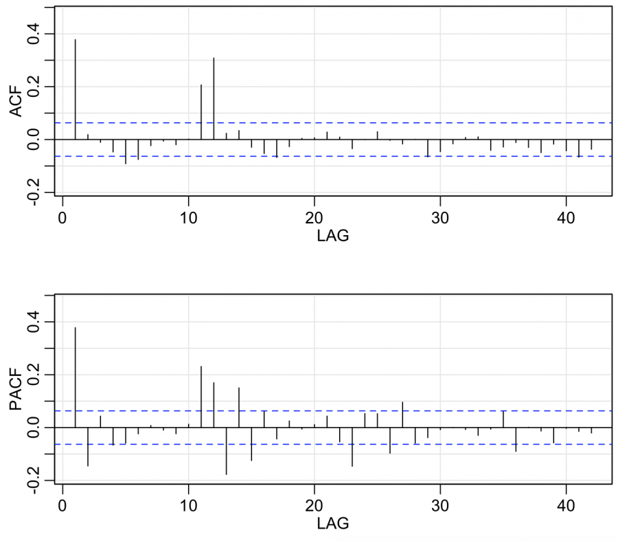
R can be used to determine and plot the PACF for this model, with \(\phi_1\)=.6 and \(\Phi_1\)=.5. That PACF (partial autocorrelation function) is:
It’s not quite what you might expect for an AR model, but it almost is. There are distinct spikes at lags 1, 12, and 13 with a bit of action coming before lag 12. Then, it cuts off after lag 13.
R commands were
thepacf=ARMAacf (ar = c(.6,0,0,0,0,0,0,0,0,0,0,.5,-.30),lag.max=30,pacf=T)
plot (thepacf,type="h")
Identifying a Seasonal Model Section
- Step 1: Do a time series plot of the data.
Examine it for features such as trend and seasonality. You’ll know that you’ve gathered seasonal data (months, quarters, etc.,) so look at the pattern across those time units (months, etc.) to see if there is indeed a seasonal pattern.
- Step 2: Do any necessary differencing.
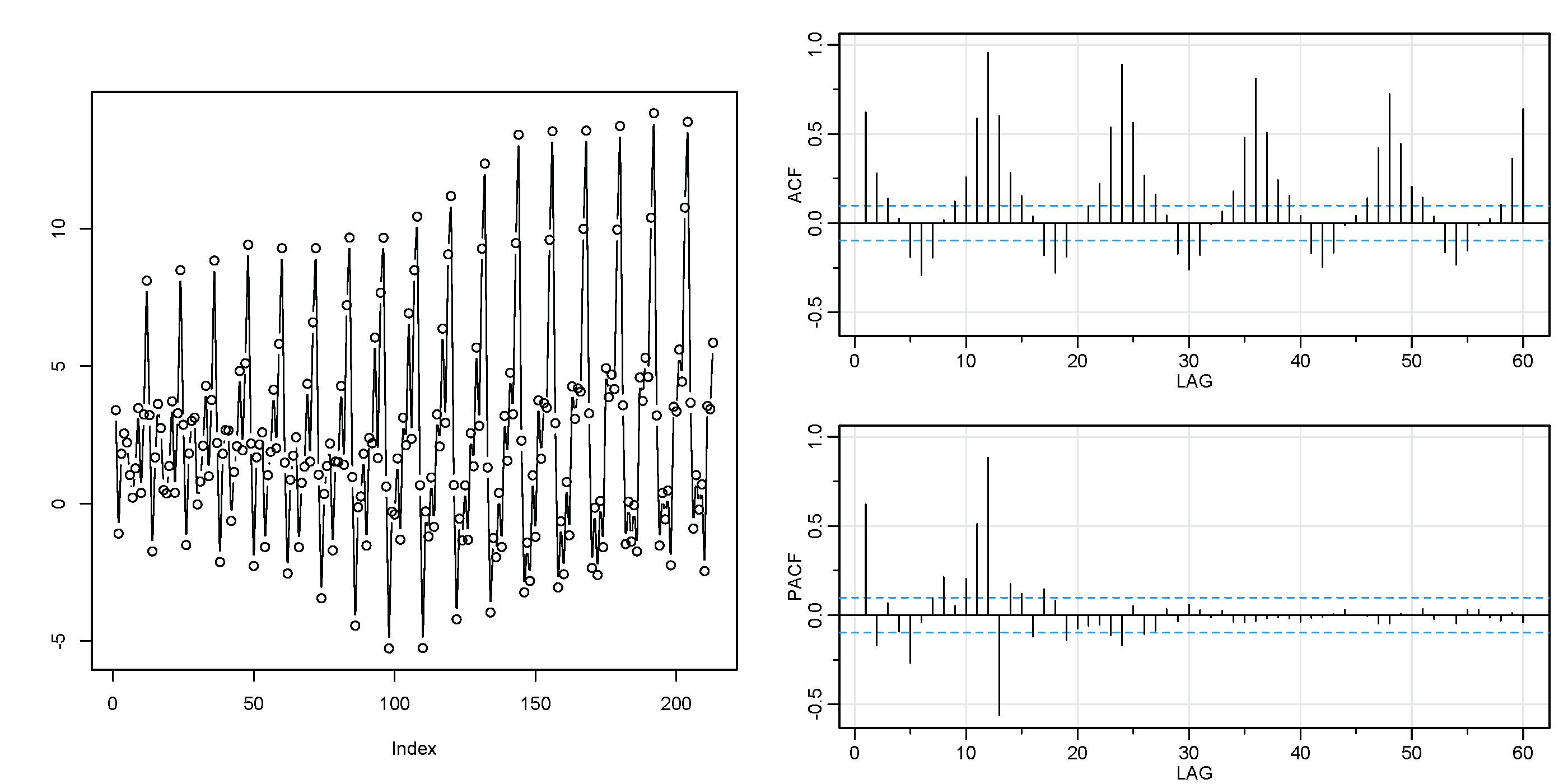
- If there is seasonality and no trend, then take a difference of lag S. For instance, take a 12th difference for monthly data with seasonality. Seasonality will appear in the ACF by tapering slowly at multiples of S. (View theTS plot and ACF/PACF plots
for an example of data that requires a seasonal difference. Note that the TS plot shows a clear seasonal pattern that repeats over 12 time points. Seasonal differences are supported in the ACF/PACF of the original data because the first seasonal lag in the ACF is close to 1 and decays slowly over multiples of S=12. Once seasonal differences are taken, the ACF/PACF plots of twelfth differences support a seasonal AR(1) pattern.)TS plot and ACF/PACF plots
 TS plot and ACF/PACF plotsACF/PACF plots
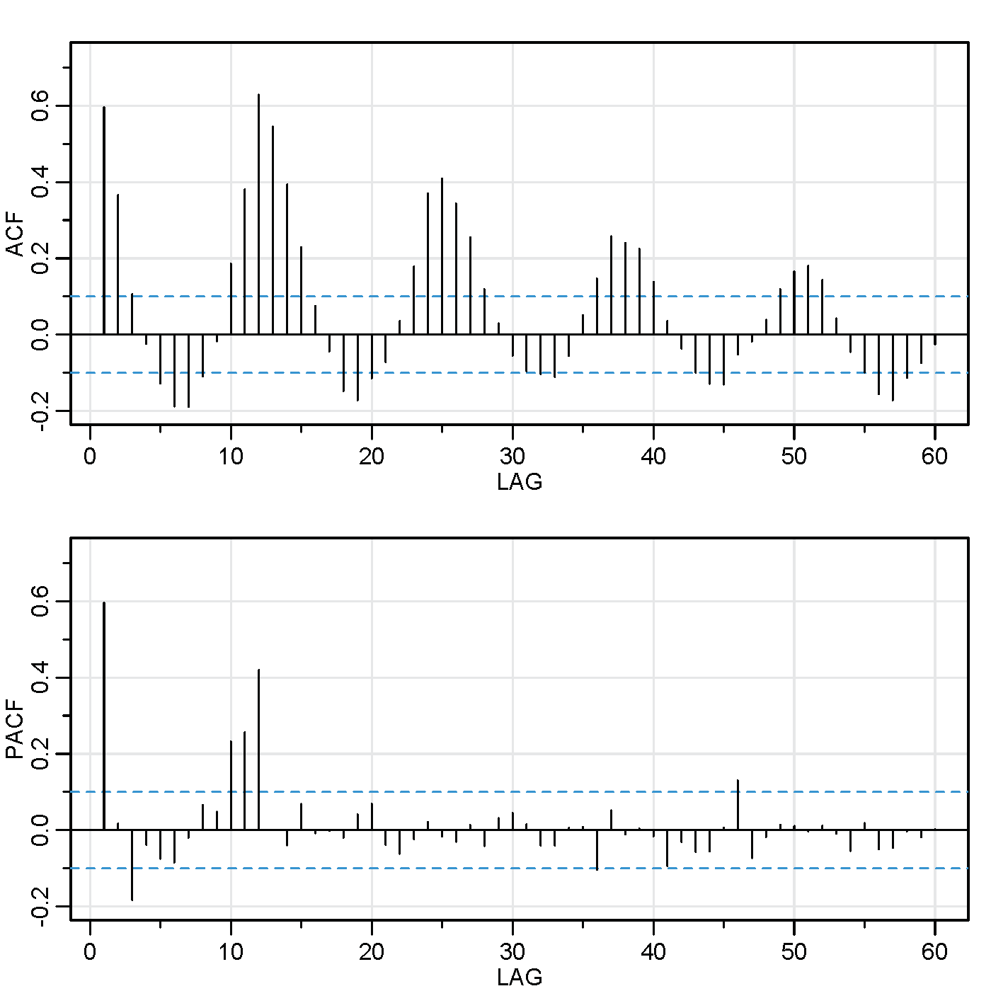 ACF/PACF plots
- If there is linear trend and no obvious seasonality, then take a first difference. If there is a curved trend, consider a transformation of the data before differencing.
- If there is both trend and seasonality, apply a seasonal difference to the data and then re-evaluate the trend. If a trend remains, then take first differences. For instance, if the series is called x, the commands in R would be:
diff12=diff(x, 12) plot(diff12) acf2(diff12) diff1and12 = diff(diff12, 1) - If there is neither obvious trend nor seasonality, don’t take any differences.
- Step 3: Examine the ACF and PACF of the differenced data (if differencing is necessary).
We’re using this information to determine possible models. This can be tricky going involving some (educated) guessing. Some basic guidance:
-
Non-seasonal terms: Examine the early lags (1, 2, 3, …) to judge non-seasonal terms. Spikes in the ACF (at low lags) with a tapering PACF indicate non-seasonal MA terms. Spikes in the PACF (at low lags) with a tapering ACF indicate possible non-seasonal AR terms.
-
Seasonal terms: Examine the patterns across lags that are multiples of S. For example, for monthly data, look at lags 12, 24, 36, and so on (probably won’t need to look at much more than the first two or three seasonal multiples). Judge the ACF and PACF at the seasonal lags in the same way you do for the earlier lags.
-
- Step 4: Estimate the model(s) that might be reasonable on the basis of step 3.
Don’t forget to include any differencing that you did before looking at the ACF and PACF. In the software, specify the original series as the data and then indicate the desired differencing when specifying parameters in the arima command that you’re using.
- Step 5: Examine the residuals (with ACF, Box-Pierce, and any other means) to see if the model seems good.
Compare AIC or BIC values to choose among several models.
If things don’t look good here, it’s back to Step 3 (or maybe even Step 2).
Example 4-3 Section
The data series are a monthly series of a measure of the flow of the Colorado River, at a particular site, for n = 600 consecutive months.
Step 1
A time series plot is
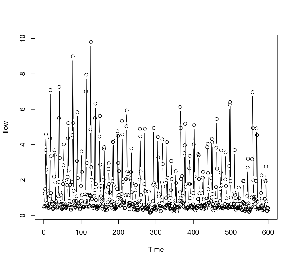
With so many data points, it’s difficult to judge whether there is seasonality. If it was your job to work on data like this, you probably would know that river flow is seasonal – perhaps likely to be higher in the late spring and early summer, due to snow runoff.
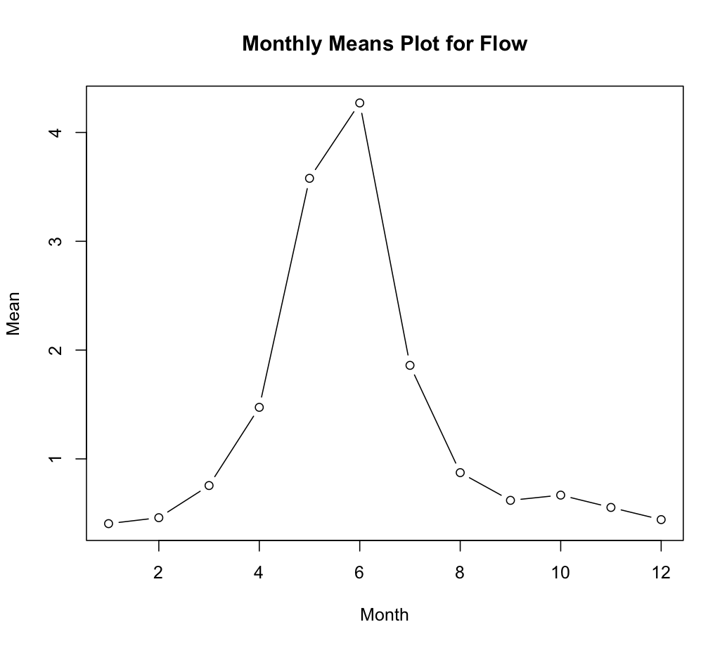
Without this knowledge, we might determine means by month of the year. Below is a plot of means for the 12 months of the year. It’s clear that there are monthly differences (seasonality).
Looking back at the time series plot, it’s hard to judge whether there’s any long run trend. If there is, it’s slight.
Steps 2 and 3
We might try the idea that there is seasonality, but no trend. To do this, we can create a variable that gives the 12th differences (seasonal differences), calculated as \(x _ { t } - x _ { t - 12}\). Then, we look at the ACF and the PACF for the 12th difference series (not the original data). Here they are:
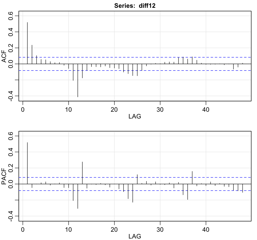
- Non-seasonal behavior: The PACF shows a clear spike at lag 1 and not much else until about lag 11. This is accompanied by a tapering pattern in the early lags of the ACF. A non-seasonal AR(1) may be a useful part of the model.
- Seasonal behavior: We look at what’s going on around lags 12, 24, and so on. In the ACF, there’s a cluster of (negative) spikes around lag 12 and then not much else. The PACF tapers in multiples of S; that is the PACF has significant lags at 12, 24, 36 and so on. This is similar to what we saw for a seasonal MA(1) component in Example 1 of this lesson.
Remembering that we’re looking at 12th differences, the model we might try for the original series is ARIMA \(( 1,0,0 ) \times ( 0,1,1 ) _ { 12 }\).
Step 4
R results for the ARIMA \(( 1,0,0 ) \times ( 0,1,1 ) _ { 12 }\):
Final Estimates of Parameters
| Type | Coef | SE Coef | T | P |
|---|---|---|---|---|
| AR 1 | 0.5149 | 0.0353 | 14.60 | 0.000 |
| SMA 12 | -0.8828 | 0.0237 | -37.25 | 0.000 |
| Constant | -0.0011 | 0.0007 | -1.63 | 0.103 |
sigma^2 estimated as 0.4681: log likelihood = -620.38, aic = 1248.76
$degrees_of_freedom
[1] 585
Step 5 (diagnostics)
The normality and Box-Pierce test results are shown in Lesson 4.2. Besides normality, things look good. The Box-Pierce statistics are all non-significant and the estimated ARIMA coefficients are statistically significant.
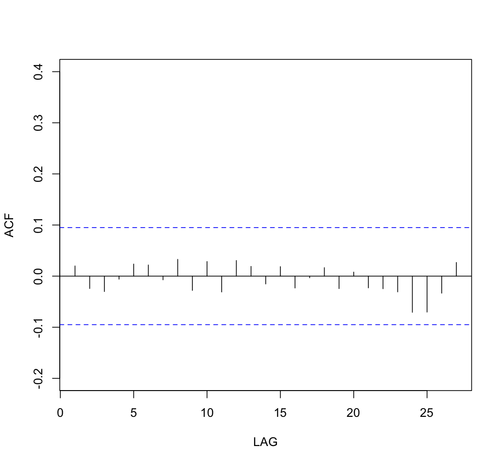
The ACF of the residuals looks good too:
What doesn’t look perfect is a plot of residuals versus fits. There’s non-constant variance.
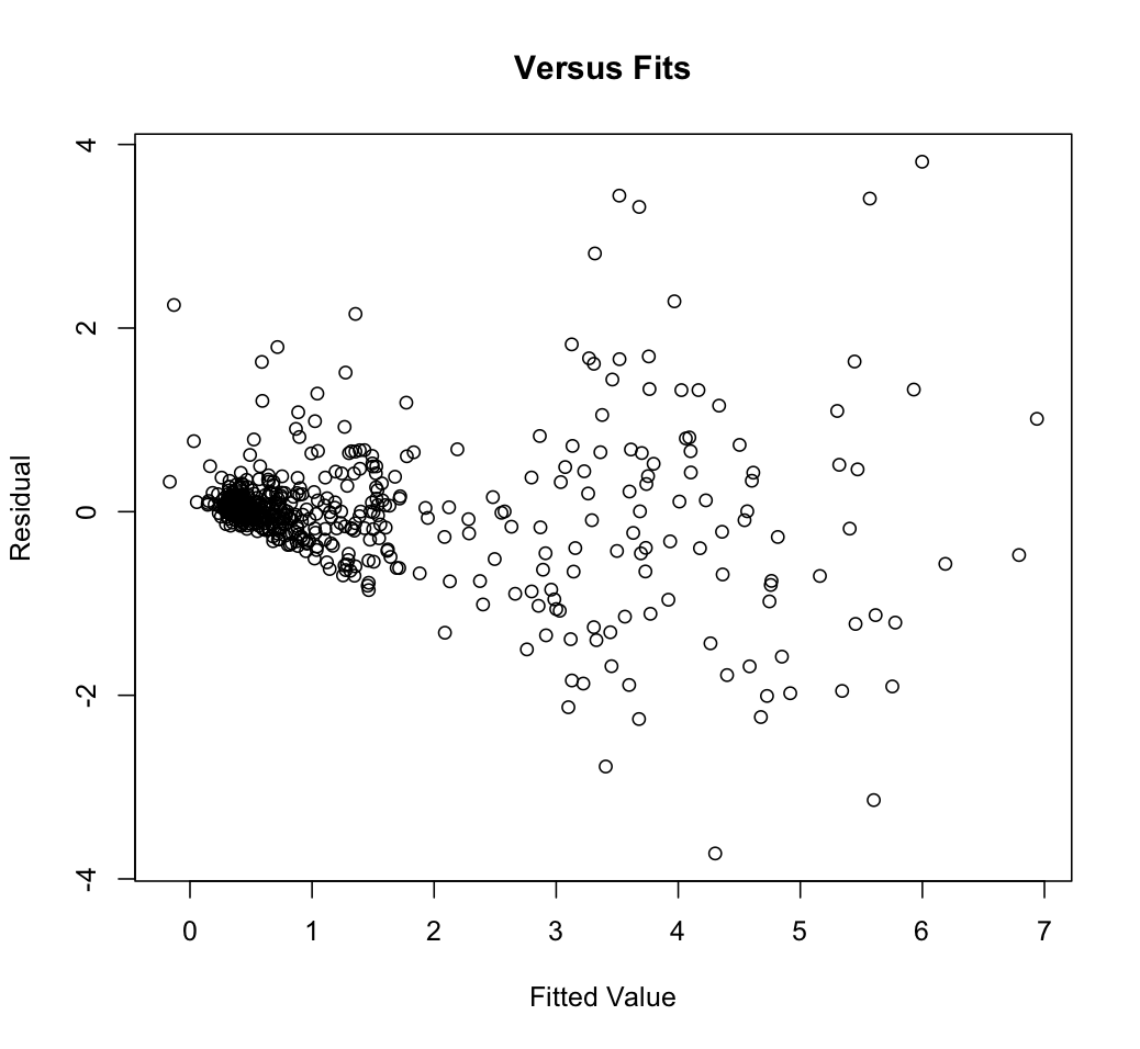
We’ve got three choices for what to do about the non-constant variance: (1) ignore it, (2) go back to step 1 and try a variance stabilizing transformation like log or square root, or (3) use an ARCH model that includes a component for changing variances. We’ll get to ARCH models later in the course.
Lesson 4.2 for this week will give R guidance and an additional example or two.
Appendix (Optional reading) Section
Only those interested in theory need to look at the following.
In Example 4-1, we promised a proof that \(\rho_{11}\) ≠ 0 for ARIMA \(( 0,0,1 ) \times ( 0,0,1 ) _ { 12 }\).
A correlation is defined as Covariance/ product of standard deviations.
The covariance between \(x_t\) and \(x _ { t - 11 } = E \left( x _ { t } - \mu \right) \left( x _ { t - 11 } - \mu \right)\).
For the model in Example 1,
\(x _ { t } - \mu = w _ { t } + \theta _ { 1 } w _ { t - 1 } + \Theta _ { 1 } w _ { t - 12 } + \theta _ { 1 } \Theta _ { 1 } w _ { t - 13 }\)
\(x _ { t - 11 } - \mu = w _ { t - 11 } + \theta _ { 1 } w _ { t - 12 } + \Theta _ { 1 } w _ { t - 23 } + \theta _ { 1 } \Theta _ { 1 } w _ { t - 24 }\)
The covariance between\(x_t\) and \(x_{t-11}\)
(2) \(\mathrm { E } \left( w _ { t } + \theta _ { 1 } w _ { t - 1 } + \Theta _ { 1 } w _ { t - 12 } + \theta _ { 1 } \Theta _ { 1 } w _ { t - 13 } \right) \left( w _ { t - 11 } + \theta _ { 1 } w _ { t - 12 } + \Theta _ { 1 } w _ { t - 23 } + \theta _ { 1 } \Theta _ { 1 } w _ { t - 24 } \right)\)
The w’s are independent errors. The expected value of any product involving w’s with different subscripts will be 0. A covariance between w’s with the same subscripts will be the variance of w.
If you inspect all possible products in expression 2, there will be one product with matching subscripts. They have lag t – 12. Thus this expected value (covariance) will be different from 0.
This shows that the lag 11 autocorrelation will be different from 0. If you look at the more general problem, you can find that only lags 1, 11, 12, and 13 have non-zero autocorrelations for the ARIMA\(( 0,0,1 ) \times ( 0,0,1 ) _ { 12 }\).
A seasonal ARIMA model incorporates both non-seasonal and seasonal factors in a multiplicative fashion.