Time series models known as ARIMA models may include autoregressive terms and/or moving average terms. In Week 1, we learned an autoregressive term in a time series model for the variable \(x_t\) is a lagged value of \(x_t\). For instance, a lag 1 autoregressive term is \(x_{t-1}\)(multiplied by a coefficient). This lesson defines moving average terms.
A moving average term in a time series model is a past error (multiplied by a coefficient).
Let \(w_t \overset{iid}{\sim} N(0, \sigma^2_w)\), meaning that the wt are identically, independently distributed, each with a normal distribution having mean 0 and the same variance.
The 1st order moving average model, denoted by MA(1) is:
\(x_t = \mu + w_t +\theta_1w_{t-1}\)
The 2nd order moving average model, denoted by MA(2) is:
\(x_t = \mu + w_t +\theta_1w_{t-1}+\theta_2w_{t-2}\)
The qth order moving average model, denoted by MA(q) is:
\(x_t = \mu + w_t +\theta_1w_{t-1}+\theta_2w_{t-2}+\dots + \theta_qw_{t-q}\)
Many textbooks and software programs define the model with negative signs before the \(\theta\) terms. This doesn’t change the general theoretical properties of the model, although it does flip the algebraic signs of estimated coefficient values and (unsquared) \(\theta\) terms in formulas for ACFs and variances. You need to check your software to verify whether negative or positive signs have been used in order to correctly write the estimated model. R uses positive signs in its underlying model, as we do here.
Theoretical Properties of a Time Series with an MA(1) Model
- Mean is \(E(x_t)=\mu\)
- Variance is \(Var(x_t)= \sigma^2_w(1+\theta^2_1)\)
- Autocorrelation function (ACF) is:
\(\rho_1 = \dfrac{\theta_1}{1+\theta^2_1}, \text{ and } \rho_h = 0 \text{ for } h \ge 2\)
That the only nonzero value in the theoretical ACF is for lag 1. All other autocorrelations are 0. Thus a sample ACF with a significant autocorrelation only at lag 1 is an indicator of a possible MA(1) model.
For interested students, proofs of these properties are in the appendix.
Example 2-1 Section
Suppose that an MA(1) model is \(x_t=10+w_t+.7w_{t-1}\), where \(w_t \overset{iid}{\sim} N(0,1)\). Thus the coefficient \(\theta_1=0.7\). The theoretical ACF is given by:
\(\rho_1 = \dfrac{0.7}{1+0.7^2} = 0.4698, \text{ and } \rho_h = 0 \text{ for all lags } h \ge 2\)
A plot of this ACF follows:
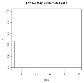
The plot just shown is the theoretical ACF for an MA(1) with \(\theta_1=0.7\). In practice, a sample won’t usually provide such a clear pattern. Using R, we simulated n = 100 sample values using the model \(x_t=10+w_t+.7w_{t-1}\) where \(w_t \overset{iid}{\sim} N(0,1)\). For this simulation, a time series plot of the sample data follows. We can’t tell much from this plot.
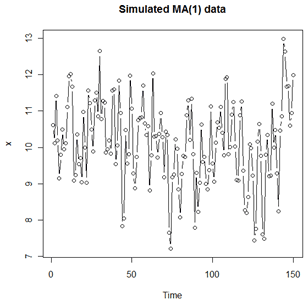
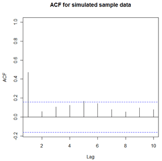
The sample ACF for the simulated data follows. We see a “spike” at lag 1 followed by generally non-significant values for lags past 1. Note that the sample ACF does not exactly match the theoretical pattern of the underlying MA(1), which is that all autocorrelations for lags above lag 1 equal zero. A different sample would have a slightly different sample ACF shown below, but would likely have the same broad features.
Theoretical Properties of a Time Series with an MA(2) Model Section
For the MA(2) model, theoretical properties are the following:
- Mean is \(E(x_t)=\mu\)
- Variance is \(Var(x_t)=\sigma^2_w(1+\theta^2_1+\theta^2_2)\)
- Autocorrelation function (ACF) is:
\( \rho_1 = \dfrac{\theta_1+\theta_1\theta_2}{1+\theta^2_1 +\theta^2_2}, \text{ } \rho_2 = \dfrac{\theta_2}{1+\theta^2_1 +\theta^2_2}, \text{ and } \rho_h = 0 \text{ for } h \ge 3 \)
The only nonzero values in the theoretical ACF are for lags 1 and 2. Autocorrelations for higher lags are 0. So, a sample ACF with significant autocorrelations at lags 1 and 2, but non-significant autocorrelations for higher lags indicates a possible MA(2) model.
Example 2-2 Section
Consider the MA(2) model \(x_t=10+w_t+.5w_{t-1}+.3w_{t-2}\), where \(w_t \overset{iid}{\sim} N(0,1)\). The coefficients are \(\theta_1=0.5\) and \(\theta_2= 0.3\). Because this is an MA(2), the theoretical ACF will have nonzero values only at lags 1 and 2.
Values of the two nonzero autocorrelations are:
\(\rho_1 = \dfrac{0.5+0.5 \times 0.3}{1+0.5^2 +0.3^2} = 0.4851 \text{ and } \rho_2 = \dfrac{0.3}{1+0.5^2 +0.3^2}= 0.2239 \)
A plot of the theoretical ACF follows:
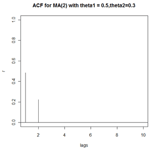
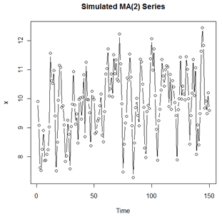
As nearly always is the case, sample data won’t behave quite so perfectly as theory. We simulated n = 150 sample values for the model \(x_t=10+w_t+.5w_{t-1}+.3w_{t-2}\), where \(w_t \overset{iid}{\sim} N(0,1)\). The time series plot of the data follows. As with the time series plot for the MA(1) sample data, you can’t tell much from it.
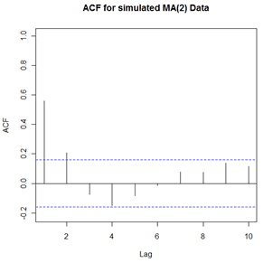
The sample ACF for the simulated data follows. The pattern is typical for situations where an MA(2) model may be useful. There are two statistically significant “spikes” at lags 1 and 2 followed by non-significant values for other lags. Note that due to sampling error, the sample ACF did not match the theoretical pattern exactly.
ACF for General MA(q) Models Section
A property of MA(q) models in general is that there are nonzero autocorrelations for the first q lags and autocorrelations = 0 for all lags > q.
Non-uniqueness of connection between values of \(\theta_1\) and \(\rho_1\) in MA(1) Model.
In the MA(1) model, for any value of \(\theta_1\), the reciprocal \(1/\theta_1\) gives the same value for:
\(\rho_1 = \dfrac{\theta_1}{1+\theta^2_1}\)
As an example, use +0.5 for \(\theta_1\), and then use 1/(0.5) = 2 for \(\theta_1\). You’ll get \(\rho_1 = 0.4\) in both instances.
To satisfy a theoretical restriction called invertibility, we restrict MA(1) models to have values with absolute value less than 1. In the example just given, \(\theta_1 = 0.5\) will be an allowable parameter value, whereas \(\theta_1 = 1/0.5 = 2\) will not.
Invertibility of MA models
An MA model is said to be invertible if it is algebraically equivalent to a converging infinite order AR model. By converging, we mean that the AR coefficients decrease to 0 as we move back in time.
Invertibility is a restriction programmed into time series software used to estimate the coefficients of models with MA terms. It’s not something that we check for in the data analysis. Additional information about the invertibility restriction for MA(1) models is given in the appendix.
For a MA(q) model with a specified ACF, there is only one invertible model. The necessary condition for invertibility is that the \(\theta\) coefficients have values such that the equation \(1-\theta_1y-...-\theta_qy^q=0\) has solutions for \(y\) that fall outside the unit circle.
R Code for the Examples Section
In Example 1, we plotted the theoretical ACF of the model \(x_t=10+w_t+.7w_{t-1}\), and then simulated n = 150 values from this model and plotted the sample time series and the sample ACF for the simulated data. The R commands used to plot the theoretical ACF were:
acfma1=ARMAacf(ma=c(0.7), lag.max=10) # 10 lags of ACF for MA(1) with theta1 = 0.7
lags=0:10 #creates a variable named lags that ranges from 0 to 10.
plot(lags,acfma1,xlim=c(1,10), ylab="r",type="h", main = "ACF for MA(1) with theta1 = 0.7")
abline(h=0) #adds a horizontal axis to the plot
The first command determines the ACF and stores it in an object named acfma1 (our choice of name).
The plot command (the 3rd command) plots lags versus the ACF values for lags 1 to 10. The ylab parameter labels the y-axis and the "main" parameter puts a title on the plot.
To see the numerical values of the ACF simply use the command acfma1.
The simulation and plots were done with the following commands:
xc=arima.sim(n=150, list(ma=c(0.7))) #Simulates n = 150 values from MA(1)
x=xc+10 # adds 10 to make mean = 10. Simulation defaults to mean = 0.
plot(x,type="b", main="Simulated MA(1) data")
acf(x, xlim=c(1,10), main="ACF for simulated sample data")
In Example 2, we plotted the theoretical ACF of the model \(x_t=10+w_t+.5w_{t-1}+.3w_{t-2}\), and then simulated n = 150 values from this model and plotted the sample time series and the sample ACF for the simulated data. The R commands used were:
acfma2=ARMAacf(ma=c(0.5,0.3), lag.max=10)
acfma2
lags=0:10
plot(lags,acfma2,xlim=c(1,10), ylab="r",type="h", main = "ACF for MA(2) with theta1 = 0.5,theta2=0.3")
abline(h=0)
xc=arima.sim(n=150, list(ma=c(0.5, 0.3)))
x=xc+10
plot(x, type="b", main = "Simulated MA(2) Series")
acf(x, xlim=c(1,10), main="ACF for simulated MA(2) Data")
Appendix: Proof of Properties of MA(1) Section
For interested students, here are proofs for theoretical properties of the MA(1) model.
The 1st order moving average model , denoted by MA(1) is \(x_t=\mu+w_t+\theta_1w_{t-1}\), where \(w_t \overset{iid}{\sim} N(0,\sigma^2_w)\).
Mean: \( E(x_t)=E(\mu + w_t + \theta_1 w_{t-1} ) = \mu + 0 + (\theta_1)(0) = \mu \)
Variance: \(\text{Var}(x_t) = \text{Var} (\mu + w_t + \theta_1 w_{t-1}) = 0 + \text{Var}(w_t) + \text{Var}(\theta_1w_{t-1}) = \sigma^2_w + \theta^2_1\sigma^2_w = (1+\theta^2_1)\sigma^2_w\)
ACF: Consider the covariance between \(x_t\) and \(x_{t-h}\). This is \(E(x_t-\mu)(x_{t-h}-\mu)\), which equals
\(E[(w_t + \theta_1w_{t-1})(w_{t-h}+\theta_1w_{t-h-1})] = E[w_tw_{t-h} + \theta_1w_{t-1}w_{t-h} +\theta_1w_tw_{t-h-1}+\theta^2_1 w_{t-1}w_{t-h-1}]\)
When \(h=1\), the previous expression = \(\theta_1 \sigma_w^2\). For any \(h \ge 2\), the previous expression = 0. The reason is that, by definition of independence of the \(w_t\), \(E(w_k w_k)=0\) for any \(k \ne j \). Further, because the \(w_t\) have mean 0, \(E(w_k w_k)=E(w_j^2)=\sigma_w^2\).
For a time series,
\(\rho_h = \dfrac{\text{Covariance for lag h}}{\text{Variance}}\)
Apply this result to get the ACF given above.
Invertibility Restriction:
An invertible MA model is one that can be written as an infinite order AR model that converges so that the AR coefficients converge to 0 as we move infinitely back in time. We’ll demonstrate invertibility for the MA(1) model.
The MA(1) model can be written as \(x_t-\mu=w_t+\theta_1 w_{t-1}\).
If we let \(z_t=x_t-\mu\), then the MA(1) model is
(1) \(z_t = w_t +\theta_1w_{t-1}\).
At time \(t-1\), the model is \(z_{t-1}=w_{t-1}+\theta_1 w_{t-2}\) which can be reshuffled to
(2) \(w_{t-1} = z_{t-1}-\theta_1w_{t-2}\).
We then substitute relationship (2) for \(w_{t-1}\) in equation (1)
(3) \(z_t = w_t +\theta_1(z_{t-1}-\theta_1w_{t-2}) = w_t +\theta_1z_{t-1} -\theta^2w_{t-2}\)
At time \(t-2\), equation (2) becomes
(4) \(w_{t-2} = z_{t-2}-\theta_1w_{t-3}\).
We then substitute relationship (4) for \(w_{t-2}\) in equation (3)
\(z_t = w_t +\theta_1 z_{t-1}-\theta^2_1w_{t-2} = w_t + \theta_1z_{t-1} -\theta^2_1(z_{t-2}-\theta_1w_{t-3}) = w_t +\theta_1z_{t-1} -\theta_1^2z_{t-2}+\theta^3_1w_{t-3}\)
If we were to continue (infinitely), we would get the infinite order AR model
\(z_t = w_t +\theta_1 z_{t-1} - \theta^2_1z_{t-2} +\theta^3_1z_{t-3}-\theta^4_1z_{t-4}+\dots \)
However, that if \(\lvert\theta_1\rvert \ge 1\), the coefficients multiplying the lags of \(z\) will increase (infinitely) in size as we move back in time. To prevent this, we need \(\lvert\theta_1\rvert < 1\). This is the condition for an invertible MA(1) model.
Infinite Order MA model
In week 3, we’ll see that an AR(1) model can be converted to an infinite order MA model:
\(x_t -\mu = w_t +\phi_1w_{t-1}+\phi^2_1w_{t-2} + \dots + \phi^k_1 w_{t-k} +\dots = \sum_{j=0}^{\infty} \phi^j_1w_{t-j}\)
This summation of past white noise terms is known as the causal representation of an AR(1). In other words, \(x_t\) is a special type of MA with an infinite number of terms going back in time. This is called an infinite order MA or MA(\(\infty \)). A finite order MA is an infinite order AR and any finite order AR is an infinite order MA.
Recall in Week 1, we noted that a requirement for a stationary AR(1) is that \(\lvert\phi_1\rvert< 1\). Let’s calculate the \(\text{Var}(x_t)\) using the causal representation.
\(\text{Var}(x_t) = \text{Var} \left(\sum_{j=0}^{\infty} \phi^j_1w_{t-j} = \sum_{j=0}^{\infty}\text{Var}(\phi^j_1w_{t-j}) = \sum_{j=0}^{\infty}\phi^{2j}_1\sigma^2_w = \sigma^2_w \sum_{j=0}^{\infty}\phi^{2j}_1 = \frac{\sigma^2_w}{1-\phi^2_1} \right)\)
This last step uses a basic fact about geometric series that requires \(\lvert\phi_1\rvert <1\); otherwise the series diverges.