In general, a partial correlation is a conditional correlation. It is the correlation between two variables under the assumption that we know and take into account the values of some other set of variables. For instance, consider a regression context in which y is the response variable and \(x_1\), \(x_2\), and \(x_3\) are predictor variables. The partial correlation between y and \(x_3\) is the correlation between the variables determined taking into account how both y and \(x_3\) are related to \(x_1\) and \(x_2\).
In regression, this partial correlation could be found by correlating the residuals from two different regressions:
- Regression in which we predict y from \(x_1\) and \(x_2\),
- regression in which we predict \(x_3\) from \(x_1\) and \(x_2\). Basically, we correlate the “parts” of y and \(x_3\) that are not predicted by \(x_1\) and \(x_2\).
More formally, we can define the partial correlation just described as
\(\dfrac{\text{Covariance}(y, x_3|x_1, x_2)}{\sqrt{\text{Variance}(y|x_1, x_2)\text{Variance}(x_3| x_1, x_2)}}\)
That this is also how the parameters of a regression model are interpreted. Think about the difference between interpreting the regression models:
\(y = \beta_0 + \beta_1x^2 \text{ and } y = \beta_0+\beta_1x+\beta_2x^2\)
In the first model, \(\beta_1\) can be interpreted as the linear dependency between \(x^2\) and y. In the second model, \(\beta_2\) would be interpreted as the linear dependency between \(x^2\) and y WITH the dependency between x and y already accounted for.
For a time series, the partial autocorrelation between \(x_{t}\) and \(x_{t-h}\) is defined as the conditional correlation between \(x_{t}\) and \(x_{t-h}\), conditional on \(x_{t-h+1}\), ... , \(x_{t-1}\), the set of observations that come between the time points \(t\) and \(t-h\).
- The 1st order partial autocorrelation will be defined to equal the 1st order autocorrelation.
- The 2nd order (lag) partial autocorrelation is
\(\dfrac{\text{Covariance}(x_t, x_{t-2}| x_{t-1})}{\sqrt{\text{Variance}(x_t|x_{t-1})\text{Variance}(x_{t-2}|x_{t-1})}}\)
This is the correlation between values two time periods apart conditional on knowledge of the value in between. (By the way, the two variances in the denominator will equal each other in a stationary series.)
- The 3rd order (lag) partial autocorrelation is
\(\dfrac{\text{Covariance}(x_t, x_{t-3}| x_{t-1}, x_{t-2})}{\sqrt{\text{Variance}(x_t|x_{t-1},x_{t-2})\text{Variance}(x_{t-3}|x_{t-1},x_{t-2})}}\)
And, so on, for any lag.
Typically, matrix manipulations having to do with the covariance matrix of a multivariate distribution are used to determine estimates of the partial autocorrelations.
Some Useful Facts About PACF and ACF Patterns Section
Identification of an AR model is often best done with the PACF.
- For an AR model, the theoretical PACF “shuts off” past the order of the model. The phrase “shuts off” means that in theory the partial autocorrelations are equal to 0 beyond that point. Put another way, the number of non-zero partial autocorrelations gives the order of the AR model. By the “order of the model” we mean the most extreme lag of x that is used as a predictor.
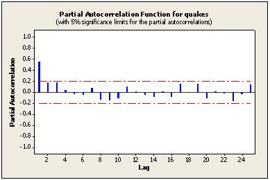
Example: In Lesson 1.2, we identified an AR(1) model for a time series of annual numbers of worldwide earthquakes having a seismic magnitude greater than 7.0. Following is the sample PACF for this series. Note that the first lag value is statistically significant, whereas partial autocorrelations for all other lags are not statistically significant. This suggests a possible AR(1) model for these data.

Identification of an MA model is often best done with the ACF rather than the PACF.
For an MA model, the theoretical PACF does not shut off, but instead tapers toward 0 in some manner. A clearer pattern for an MA model is in the ACF. The ACF will have non-zero autocorrelations only at lags involved in the model.
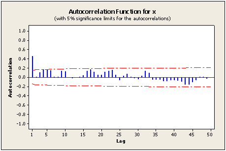
Lesson 2.1 included the following sample ACF for a simulated MA(1) series. Note that the first lag autocorrelation is statistically significant whereas all subsequent autocorrelations are not. This suggests a possible MA(1) model for the data.
The model used for the simulation was \(x_t=10+w_t+0.7w_{t-1}\). In theory, the first lag autocorrelation \(\theta_1 / (1+\theta_1^2) = .7/(1+.7^2) = .4698 \) and autocorrelations for all other lags = 0.

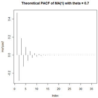
The underlying model used for the MA(1) simulation in Lesson 2.1 was \(x_t=10+w_t+0.7w_{t-1}\). Following is the theoretical PACF (partial autocorrelation) for that model. Note that the pattern gradually tapers to 0.

The PACF just shown was created in R with these two commands:
ma1pacf = ARMAacf(ma = c(.7),lag.max = 36, pacf=TRUE)
plot(ma1pacf,type="h", main = "Theoretical PACF of MA(1) with theta = 0.7")