ARIMA models, also called Box-Jenkins models, are models that may possibly include autoregressive terms, moving average terms, and differencing operations. Various abbreviations are used:
- When a model only involves autoregressive terms it may be referred to as an AR model. When a model only involves moving average terms, it may be referred to as an MA model.
- When no differencing is involved, the abbreviation ARMA may be used.
This week we’re only considering non-seasonal models. We’ll expand our toolkit to include seasonal models next week.
Specifying the Elements of the Model Section
In most software programs, the elements in the model are specified in the order (AR order, differencing, MA order). As examples,
A model with (only) two AR terms would be specified as an ARIMA of order (2,0,0).
A MA(2) model would be specified as an ARIMA of order (0,0,2).
A model with one AR term, a first difference, and one MA term would have order (1,1,1).
For the last model, ARIMA (1,1,1), a model with one AR term and one MA term is being applied to the variable \(Z _ { t } = X _ { t } - X _ { t - 1 }\). A first difference might be used to account for a linear trend in the data.
The differencing order refers to successive first differences. For example, for a difference order = 2 the variable analyzed is \(z _ { t } = \left( x _ { t } - x _ { t - 1 } \right) - \left( x _ { t - 1 } - x _ { t - 2 } \right)\), the first difference of first differences. This type of difference might account for a quadratic trend in the data.
Identifying a Possible Model Section
Three items should be considered to determine the first guess at an ARIMA model: a time series plot of the data, the ACF, and the PACF.
-
Time series plot of the observed series
In Lesson 1.1, we discussed what to look for: possible trend, seasonality, outliers, constant variance or nonconstant variance.
Note!
Nonconstant variance in a series with no trend may have to be addressed with something like an ARCH model which includes a model for changing variation over time. We’ll cover ARCH models later in the course.- You won’t be able to spot any particular model by looking at this plot, but you will be able to see the need for various possible actions.
- If there’s an obvious upward or downward linear trend, a first difference may be needed. A quadratic trend might need a 2nd order difference (as described above). We rarely want to go much beyond two. In those cases, we might want to think about things like smoothing, which we will cover later in the course. Over-differencing can cause us to introduce unnecessary levels of dependency (difference white noise to obtain an MA(1)–difference again to obtain an MA(2), etc.)
- For data with a curved upward trend accompanied by increasing variance, you should consider transforming the series with either a logarithm or a square root.
-
ACF and PACF
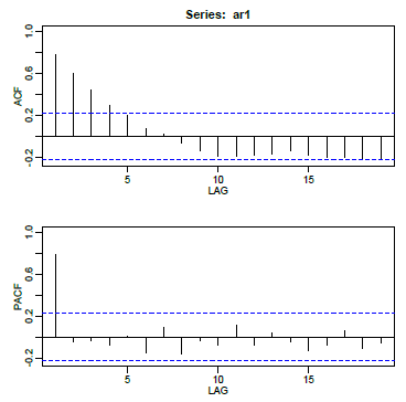
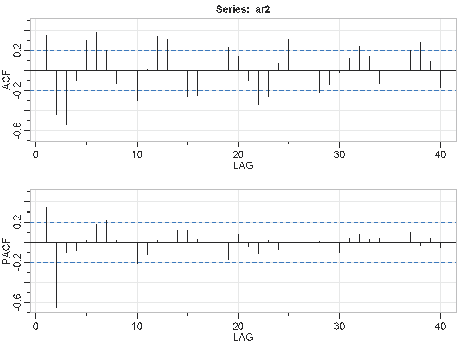
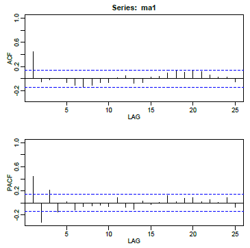
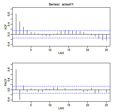
The ACF and PACF should be considered together. It can sometimes be tricky going, but a few combined patterns do stand out. Note that each pattern includes a discussion of both plots and so you should always describe how both plots suggest a model. (These are listed in Table 3.1 of the book in Section 3.3).
- AR models have theoretical PACFs with non-zero values at the AR terms in the model and zero values elsewhere. The ACF will taper to zero in some fashion.
An AR(1) model has a single spike in the PACF and an ACF with a pattern
\(\rho_k = \phi_1^k\)
- An AR(2) has two spikes in the PACF and a sinusoidal ACF that converges to 0.
- MA models have theoretical ACFs with non-zero values at the MA terms in the model and zero values elsewhere. The PACF will taper to zero in some fashion.
- ARMA models (including both AR and MA terms) have ACFs and PACFs that both tail off to 0. These are the trickiest because the order will not be particularly obvious. Basically you just have to guess that one or two terms of each type may be needed and then see what happens when you estimate the model.
- If the ACF does not tail off, but instead has values that stay close to 1 over many lags, the series is non-stationary and differencing will be needed. Try a first difference and then look at the ACF and PACF of the differenced data.
- If the series autocorrelations are non-significant, then the series is random (white noise; the ordering matters, but the data are independent and identically distributed.) You’re done at that point.
- If first differences were necessary and all the differenced autocorrelations are non-significant, then the original series is called a random walk and you are done. (A possible model for a random walk is \(x_t=\delta+x_{t-1}+w_t\). The data are dependent and are not identically distributed; in fact both the mean and variance are increasing through time.)
Note!
You might also consider examining plots of \(x_t\) versus various lags of \(x_t\) . - AR models have theoretical PACFs with non-zero values at the AR terms in the model and zero values elsewhere. The ACF will taper to zero in some fashion.
Estimating and Diagnosing a Possible Model Section
After you’ve made a guess (or two) at a possible model, use software such as R, Minitab, or SAS to estimate the coefficients. Most software will use maximum likelihood estimation methods to make the estimates. Once the model has been estimated, do the following.
- Look at the significance of the coefficients. In R, sarima provides p-values and so you may simply compare the p-value to the standard 0.05 cut-off. The arima command does not provide p-values and so you can calculate a t-statistic: \(t\) = estimated coeff. / std. error of coeff. Recall that \(t_{\alpha,df}\) is the Student \(t\)-value with area \("\alpha"\) to the right of \(t_{\alpha,df}\) on df degrees of freedom. If \(\lvert t \rvert > t_{0.025,n-p-q-1}\), then the estimated coefficient is significantly different from 0. When n is large, you may compare estimated coeff. / std. error of coeff to 1.96.
- Look at the ACF of the residuals. For a good model, all autocorrelations for the residual series should be non-significant. If this isn’t the case, you need to try a different model.
- Look at Box-Pierce (Ljung) tests for possible residual autocorrelation at various lags (see Lesson 3.2 for a description of this test).
- If non-constant variance is a concern, look at a plot of residuals versus fits and/or a time series plot of the residuals.
If something looks wrong, you’ll have to revise your guess at what the model might be. This might involve adding parameters or re-interpreting the original ACF and PACF to possibly move in a different direction.
What if More Than One Model Looks Okay? Section
Sometimes more than one model can seem to work for the same dataset. When that’s the case, some things you can do to decide between the models are:
- Possibly choose the model with the fewest parameters.
- Examine standard errors of forecast values. Pick the model with the generally lowest standard errors for predictions of the future.
- Compare models with regard to statistics such as the MSE (the estimate of the variance of the wt), AIC, AICc, and SIC (also called BIC). Lower values of these statistics are desirable.
AIC, AICc, and SIC (or BIC) are defined and discussed in Section 2.1 of our text. The statistics combine the estimate of the variance with values of the sample size and number of parameters in the model.
One reason that two models may seem to give about the same results is that, with the certain coefficient values, two different models can sometimes be nearly equivalent when they are each converted to an infinite order MA model. [Every ARIMA model can be converted to an infinite order MA – this is useful for some theoretical work, including the determination of standard errors for forecast errors.] We’ll see more about this in Lesson 3.2.
Example 3-1: Lake Erie Section
The Lake Erie data (eriedata.dat from Week 1 assignment. The series is n = 40 consecutive annual measurements of the level of Lake Erie in October.
Identifying the model.
A time series plot of the data is the following:
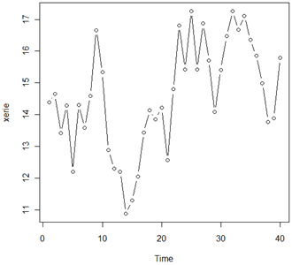
There's a possibility of some overall trend, but it might look that way just because there seemed to be a big dip around the 15th time or so. We'll go ahead without worrying about trend.
The ACF and the PACF of the series are the following. (They start at lag 1).
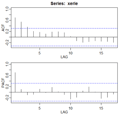
The PACF shows a single spike at the first lag and the ACF shows a tapering pattern. An AR(1) model is indicated.
Estimating the Model
We used an R script written by one of the authors of our book (Stoffer) to estimate the AR(1) model. Here's part of the output:
Coefficients:
| ar1 | xmean | |
|---|---|---|
| Estimate | 0.6909 | 14.6309 |
| Std. Error | 0.1094 | 0.5840 |
sigma^2 estimated as 1.447: log likelihood = -64.47,
\$AIC
[1] 3.373462
\$AICc
[1] 3.38157
\$BIC
[1] 3.500128
Where the coefficients are listed, notice the heading "xmean." This is giving the estimated mean of the series based on this model, not the intercept. The model used in the software is of the form \((x_t - \mu) = \phi_1(x_{t-1}-\mu)+w_t\).
The estimated model can be written as (xt - 14.6309) = 0.6909(xt-1 - 14.6309) + wt.
This is equivalent to xt = 14.6309 - (14.6309*0.6909) + 0.6909xt-1 + wt = 4.522 + 0.6909xt-1 + wt.
The AR coefficient is statistically significant (z = 0.6909/0.1094 = 6.315). It's not necessary to test the mean coefficient. We know that it's not 0.
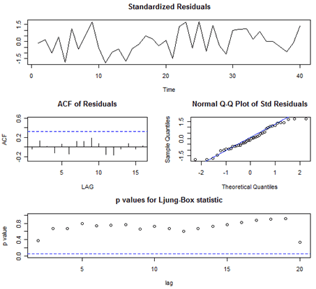
The author's routine also gives residual diagnostics in the form of several graphs. Here's that part of the output:
Interpretations of the Diagnostics
The time series plot of the standardized residuals mostly indicates that there's no trend in the residuals, no outliers, and in general, no changing variance across time.
The ACF of the residuals shows no significant autocorrelations – a good result.
The Q-Q plot is a normal probability plot. It doesn't look too bad, so the assumption of normally distributed residuals looks okay.
The bottom plot gives p-values for the Ljung-Box-Pierce statistics for each lag up to 20. These statistics consider the accumulated residual autocorrelation from lag 1 up to and including the lag on the horizontal axis. The dashed blue line is at .05. All p-values are above it. That's a good result. We want non-significant values for this statistic when looking at residuals. Read Lesson 3.2 of this week for more about the Ljung–Box-Pierce statistic.
All in all, the fit looks good. There's not much need to continue, but just to show you how things looks when incorrect models are used, we will present another model.
Output for a Wrong Model
Suppose that we had misinterpreted the ACF and PACF of the data and had tried an MA(1) model rather than the AR(1) model.
Here's the output:
Coefficients:
| ma1 | xmean | |
|---|---|---|
| Estimate | 0.5570 | 14.5881 |
| Std. Error | 0.1251 | 0.3337 |
sigma^2 estimated as 1.870: log likelihood = -69.46
\$AIC
[1] 3.622905
\$AICc
[1] 3.631013
\$BIC
[1] 3.74957
The MA(1) coefficient is significant (you can check it), but mostly this looks worse than the statistics for the right model. The estimate of the variance is 1.87, compared to 1.447 for the AR(1) model. The AIC and BIC statistics are higher for the MA(1) than for the AR(1). That's not good.
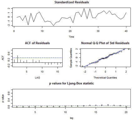
The diagnostic graphs aren't good for the MA(1). The ACF has a significant spike at lag 2 and several of the Ljung-Box-Pierce p-values are below .05. We don't want them there. So, the MA(1) isn't a good model.
A Model with One Too Many Coefficients:
Suppose we try a model (still the Lake Erie Data) with one AR term and one MA term. Here's some of the output:
| ar1 | ma1 | xmean | |
|---|---|---|---|
| Estimate | 0.7362 | -0.0909 | 14.6307 |
| Std. Error | 0.1362 | 0.1969 | 0.6142 |
sigma^2 estimated as 1.439: log likelihood = -64.36,
\$AIC
[1] 3.418224
\$AICc
[1] 3.434891
\$BIC
[1] 3.587112
The MA(1) coefficient is not significant (z = -0.0909/.1969=-0.4617 is less than 1.96 in absolute value). The MA(1) term could be dropped so that takes us back to the AR(1). Also, the estimate of the variance is barely better than the estimate for the AR(1) model and the AIC and BIC statistics are higher for the ARMA(1,1) than for the AR(1).
Example 3-2: Parameter Redundancy Section
Suppose that the model for your data is white noise. If this is true for every \(t\), then it is true for \(t-1\) as well, in other words:
\(x_t = w_t\)
\(x_{t-1} = w_{t-1}\)
Let's multiply both sides of the second equation by 0.5:
\(0.5x_{t-1} = 0.5w_{t-1}\)
Next, we will move both terms over to one side:
\(0 = -0.5x_{t-1} + 0.5w_{t-1}\)
Because the data is white noise, \(x_t=w_t\), so we can add \(x_t\) to the left side and \(w_t\) to the right side:
\(x_t = -0.5x_{t-1} + w_t + 0.5w_{t-1}\)
This is an ARMA(1, 1)! The problem is that we know it is white noise because of the original equations. If we looked at the ACF what would we see? You would see the ACF corresponding to white noise, a spike at zero and then nothing else. This also means if we take the white noise process and you try to fit in an ARMA(1, 1), R will do it and will come up with coefficients that looks something like what we have above. This is one of the reasons why we need to look at the ACF and the PACF plots and other diagnostics. We prefer a model with the fewest parameters. This example also says that for certain parameter values, ARMA models can appear very similar to one another.
R Code for Example 3-1 Section
Here’s how we accomplished the work for the example in this lesson.
We first loaded the astsa library discussed in Lesson 1. It’s a set of scripts written by Stoffer, one of the textbook’s authors. If you installed the astsa package during Lesson 1, then you only need the library command.
Use the command library("astsa"). This makes the downloaded routines accessible.
The session for creating Example 1 then proceeds as follows:
xerie = scan("eriedata.dat") #reads the data
xerie = ts (xerie) # makes sure xerie is a time series object
plot (xerie, type = "b") # plots xerie
acf2 (xerie) # author’s routine for graphing both the ACF and the PACF
sarima (xerie, 1, 0, 0) # this is the AR(1) model estimated with the author’s routine
sarima (xerie, 0, 0, 1) # this is the incorrect MA(1) model
sarima (xerie, 1, 0, 1) # this is the over-parameterized ARMA(1,1) model
In Lesson 3.3, we’ll discuss the use of ARIMA models for forecasting. Here’s how you would forecast for the next 4 times past the end of the series using the author’s source code and the AR(1) model for the Lake Erie data.
sarima.for(xerie, 4, 1, 0, 0) # four forecasts from an AR(1) model for the erie data
You’ll get forecasts for the next four times, the standard errors for these forecasts, and a graph of the time series along with the forecasts. More details about forecasting will be given in Lesson 3.3.
Some useful information about the author’s scripts available here.
