The basic problem we’re considering is the description and modeling of the relationship between two time series.
In the relationship between two time series (\(y_{t}\) and \(x_{t}\)), the series \(y_{t}\) may be related to past lags of the x-series. The sample cross correlation function (CCF) is helpful for identifying lags of the x-variable that might be useful predictors of \(y_{t}\).
In R, the sample CCF is defined as the set of sample correlations between \(x_{t+h}\) and \(y_{t}\) for h = 0, ±1, ±2, ±3, and so on. A negative value for \(h\) is a correlation between the x-variable at a time before \(t\) and the y-variable at time \(t\). For instance, consider \(h\) = −2. The CCF value would give the correlation between \(x_{t-2}\) and \(y_{t}\).
- When one or more \(x_{t+h}\) , with \(h\) negative, are predictors of \(y_{t}\), it is sometimes said that x leads y.
- When one or more \(x_{t+h}\), with \(h\) positive, are predictors of \(y_{t}\), it is sometimes said that x lags y.
In some problems, the goal may be to identify which variable is leading and which is lagging. In many problems we consider, though, we’ll examine the x-variable(s) to be a leading variable of the y-variable because we will want to use values of the x-variable to predict future values of y.
Thus, we’ll usually be looking at what’s happening at the negative values of \(h\) on the CCF plot.
Minitab calculates its sample CCF as the set of sample correlations between \(x_{t}\) and \(y_{t+h}\). Hence, the “x leading y” side of the plot is for \(h\) positive. That’s where x comes before y in time.
Transfer Function Models
In a full transfer function model, we model \(y_{t}\) as potentially a function of past lags of \(y_{t}\) and current and past lags of the x-variables. We also usually model the time series structure of the x-variables as well. We’ll take all of that on next week. This week we’ll just look at the use of the CCF to identify some relatively simple regression structures for modeling \(y_{t}\).
Sample CCF in R
The CCF command is
ccf(x-variable name, y-variable name)
If you wish to specify how many lags to show, add that number as an argument of the command. For instance, ccf(x,y, 50) will give the CCF for values of \(h\) = 0, ±1, …, ±50.
Example: Southern Oscillation Index and Fish Populations in the southern hemisphere.
The text describes the relationship between a measure of weather called the Southern Oscillation Index (SOI) and “recruitment,” a measure of the fish population in the southern hemisphere. The data are monthly estimates for n = 453 months. We see SOI as a potential predictor of recruit.
The data are in two different files. The CCF below was created with these commands:
soi= scan("soi.dat")
rec = scan("recruit.dat")
soi=ts (soi)
rec = ts(rec)
ccf (soi, rec)
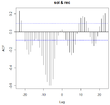
The most dominant cross correlations occur somewhere between \(h\) =−10 and about \(h\) = −4. It’s difficult to read the lags exactly from the plot, so we might want to give an object name to the ccf and then list the object contents. The following two commands will do that for our example.
ccfvalues = ccf(soi,rec)
ccfvalues
The result, showing lag (the \(h\) in xt+h) and correlation with yt :
| -23 | -22 | -21 | -20 | -19 | -18 | -17 | -16 | -15 | -14 | -13 |
| 0.235 | 0.125 | 0.000 | -0.108 | -0.198 | -0.253 | -0.222 | -0.149 | -0.092 | -0.076 | -0.103 |
| -12 | -11 | -10 | -9 | -8 | -7 | -6 | -5 | -4 | -3 | -2 |
| -0.175 | -0.267 | -0.369 | -0.476 | -0.560 | -0.598 | -0.599 | -0.527 | -0.297 | -0.146 | -0.042 |
| -1 | 0 | 1 | 2 | 3 | 4 | 5 | 6 | 7 | 8 | 9 |
| 0.011 | 0.025 | -0.013 | -0.086 | -0.154 | -0.228 | -0.259 | -0.232 | -0.144 | -0.017 | 0.094 |
| 10 | 11 | 12 | 13 | 14 | 15 | 16 | 17 | 18 | 19 | 20 |
| 0.154 | 0.174 | 0.162 | 0.118 | 0.043 | -0.057 | -0.129 | -0.156 | -0.131 | -0.049 | 0.060 |
There are nearly equal maximum values at \(h\) = −5, −6, −7, and −8 with tapering occurring in both directions from that peak.
The correlations in this region are negative, indicating that an above average value of SOI is likely to lead to a below average value of “recruit” about 6 months later. And, a below average of SOI is associated with a likely above average recruit value about 6 months later.
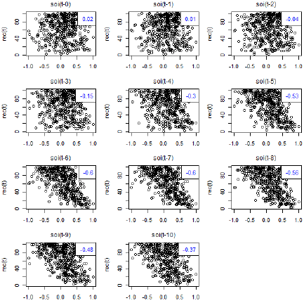
Scatterplots
In the "astsa" library that we’ve been using, Stoffer included a script that produces scatterplots of yt versus xt+h for negative \(h\) from 0 back to a lag that you specify. The command is lag2.plot.
The result of the command lag2.plot (soi, rec, 10) is shown below. In each plot, (recruit variable) is on the vertical and a past lag of SOI is on the horizontal. Correlation values are given on each plot.
Regression Models
There are a lot of models that we could try based on the CCF and lagged scatterplots for these data. For demonstration purposes, we’ll first try a multiple regression in which yt, the recruit variable, is a linear function of (past) lags 5, 6, 7, 8, 9, and 10 of the SOI variable. That model works fairly well. Following is some R output. All coefficients are statistically significant and the R-squared is about 62%.
The residuals, however, have an AR(2) structure, as seen in the graph following the regression output. We might try the method described in Lesson 8.1 to adjust for that, but we’ll take a different approach that we’ll describe after the output display.
Coefficients:
| Estimate | Std. Error | t value | Pr(>|t|) | ||
|---|---|---|---|---|---|
| (Intercept) | 69.2743 | 0.8703 | 79.601 | < 2e-16 | *** |
| soilag5 | -23.8255 | 2.7657 | -8.615 | < 2e-16 | *** |
| soilag6 | -15.3775 | 3.1651 | -4.858 | 1.65e-06 | *** |
| soilag7 | -11.7711 | 3.1665 | -3.717 | 0.000228 | *** |
| soilag8 | -11.3008 | 3.1664 | -3.569 | 0.000398 | *** |
| soilag9 | -9.1525 | 3.1651 | -2.892 | 0.004024 | ** |
| soilag10 | -16.7219 | 2.7693 | -6.038 | 3.33e-09 | *** |
Residual standard error: 17.42 on 436 degrees of freedom
(20 observations deleted due to missingness)
Multiple R-squared: 0.6251, Adjusted R-squared: 0.62
Next week we’ll discuss more about ways to interpret the CCF. One feature that will be described in more detail (with the “why”) is that a peak in a CCF followed by a tapering pattern is an indicator that lag 1 and possibly lag 2 values of the y-variable may be helpful predictors.
So, our try number 2 for a regression model will be to use lag 1 and lag 2 values of the y-variable as well as lags 5 through 10 of the x-variable as linear predictors. Here’s the outcome:
Coefficients:
| Estimate | Std. Error | t value | Pr(>|t|) | ||
|---|---|---|---|---|---|
| (Intercept) | 11.43047 | 1.33384 | 8.570 | < 2e-16 | *** |
| reclag1 | 1.25702 | 0.04316 | 29.128 | < 2e-16 | *** |
| reclag2 | -0.41946 | 0.04120 | -10.182 | < 2e-16 | *** |
| soilag5 | -21.19210 | 1.11838 | -18.949 | < 2e-16 | *** |
| soilag6 | 9.77648 | 1.56238 | 6.257 | 9.4e-10 | *** |
| soilag7 | -1.19189 | 1.32247 | -0.901 | 0.3679 | |
| soilag8 | -2.17345 | 1.30806 | -1.662 | 0.0973 | . |
| soilag9 | 0.56520 | 1.30035 | 0.435 | 0.6640 | |
| soilag10 | -2.58630 | 1.19529 | -2.164 | 0.0310 | * |
Signif. codes: 0 ‘***’ 0.001 ‘**’ 0.01 ‘*’ 0.05 ‘.’ 0.1 ‘ ’ 1
Residual standard error: 7.034 on 434 degrees of freedom
(20 observations deleted due to missingness)
Multiple R-squared: 0.9392, Adjusted R-squared: 0.938
The R-squared value has gone to about 94%. Not all sample coefficients are statistically significant. Although it’s dangerous to drop too much from a model at once, we now see that lags 7 and above are not integral predictors in the presence of the other terms. Let's drop lags 7, 8 , 9, and maybe 10 of SOI from the model. You might disagree with dropping lag 10 of SOI, but we’ll try it because it seems odd to have a “stray” term like that. .
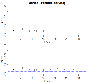
So our third attempt is to predict yt using lags 1 and 2 of itself and lags 5 and 6 of the x-variable (SOI). Here’s what happens:
Coefficients:
| Estimate | Std. Error | t value | Pr(>|t|) | ||
|---|---|---|---|---|---|
| (Intercept) | 8.78498 | 1.00171 | 8.770 | < 2e-16 | *** |
| reclag1 | 1.24575 | 0.04314 | 28.879 | < 2e-16 | *** |
| reclag2 | -0.37193 | 0.03846 | -9.670 | < 2e-16 | *** |
| soilag5 | -20.83776 | 1.10208 | -18.908 | < 2e-16 | *** |
| soilag6 | 8.55600 | 1.43146 | 5.977 | 4.68e-09 | *** |
Signif. codes: 0 ‘***’ 0.001 ‘**’ 0.01 ‘*’ 0.05 ‘.’ 0.1 ‘ ’ 1
Residual standard error: 7.069 on 442 degrees of freedom
(16 observations deleted due to missingness)
Multiple R-squared: 0.9375, Adjusted R-squared: 0.937
F-statistic: 1658 on 4 and 442 DF, p-value: < 2.2e-16
All sample coefficients are significant and the R-squared is still about 94%. The ACF and PACF of the residuals look pretty good. There’s a barely significant residual autocorrelation at lag 4 which we may or may not want to worry about.
Complications
The CCF pattern is affected by the underlying time series structures of the two variables and the trend each series has. It often (perhaps most often) is helpful to de-trend and/or take into account the univariate ARIMA structure of the x-variable before graphing the CCF. We’ll play with this a bit in the homework this week and will take it on more fully next week.
R Code Section
Here’s the full R code for this handout. The alldata=ts.intersect() command preserves proper alignment between all of the lagged variables (and defines lagged variables). The tryit=lm() commands are specifying the various regression models and saving results as named objects.
Download the data used the following code: soi.dat, recruit.dat
library(astsa)
soi= scan("soi.dat")
rec = scan("recruit.dat")
soi=ts (soi)
rec = ts(rec)
ccfvalues =ccf (soi, rec)
ccfvalues
lag2.plot (soi, rec, 10)
alldata=ts.intersect(rec,reclag1=lag(rec,-1), reclag2=lag(rec,-2), soilag5 = lag(soi,-5),
soilag6=lag(soi,-6), soilag7=lag(soi,-7), soilag8=lag(soi,-8), soilag9=lag(soi,-9),
soilag10=lag(soi,-10))
tryit = lm(rec~soilag5+soilag6+soilag7+soilag8+soilag9+soilag10, data = alldata)
summary (tryit)
acf2(residuals(tryit))
tryit2 = lm(rec~reclag1+reclag2+soilag5+soilag6+soilag7+soilag8+soilag9+soilag10,
data = alldata)
summary (tryit2)
acf2(residuals(tryit2))
tryit3 = lm(rec~reclag1+reclag2+ soilag5+soilag6, data = alldata)
summary (tryit3)
acf2(residuals(tryit3))