An Extended Overview of ANCOVA
Designed experiments often contain treatment levels that have been set with increasing numerical values. For example, consider a chemical process which is hypothesized to vary by two factors: the Reagent type (A or B), and temperature. Researchers conducted an experiment that investigates a response at 40, 50, 60, 70, and 80 degrees (F) for each of the Reagent types.
You can find the data at QuantFactorData.csv
If temperature is considered as a categorical factor, we can proceed as usual with a 2 × 5 factorial ANOVA to evaluate the null hypotheses
\(H_0 \colon \mu_A = \mu_B\)
\(H_0 \colon \mu_{40} = \mu_{50} = \mu_{60} = \mu_{70} = \mu_{80}\)
and
\(H_0\colon\) no interaction.
Although the above hypotheses compare the response means for the process carried out at different temperatures, no conclusion can be made about the trend of the response as the temperature is increased.
In general, the trend effects of a continuous predictor are modeled using a polynomial where its non-constant terms represent the different trends, such as linear, quadratic, and cubic effects. These non-constant terms in the polynomial are called trend terms.
The statistical significance of these trend terms can be tested in an ANCOVA by adding columns into the design matrix (X) of the General Linear Model (see Lesson 4 for the definition of a design matrix). These additional columns will represent the trend terms and their interaction effects with the categorical factor. Inclusion of the trend term columns will facilitate significance testing for the overall trend effects, whereas the columns representing the interactions can be utilized to compare differences of each trend effect among the categorical factor levels.
In the chemical process example, if the quantitative property of temperature is used, we can carry out an ANCOVA by fitting a polynomial regression model to express the impact of temperature on the response. If a quadratic polynomial is desired, the appropriate ANCOVA design matrix can be obtained by adding two columns representing \(temp\) and \(temp^2\) to the existing column of ones representing the reagent type A (the reference category) and the dummy variable column representing the reagent type B.
The \(temp\) and \(temp^2\) terms allow us to investigate the linear and quadratic trends, respectively. Furthermore, the inclusion of columns representing the interactions between the reagent type and the two trend terms will facilitate the testing of differences between these two trends between the two reagent types. Note also that additional columns can be added appropriately to fit a polynomial of an even higher order.
Rule: To fit a polynomial of degree n, the response should be measured at least (n+1) distinct levels of the covariate. Preliminary graphics such as scatterplots are useful in deciding the degree of the polynomial to be fitted.
Suggestion: To reduce structural multicollinearity, centering the covariate by subtracting the mean is recommended. For more details see STAT 501 - Lesson 12: Multicollinearity
Using Technology
In SAS, this process would look like this:
/*centering the covariate creating x^2 */
                data centered_quant_factor;
                set quant_factor;
                x = temp-60;
                x2 = x**2;
                run;
                proc mixed data=centered_quant_factor method=type1;
                class reagent;
                model product=reagent x x2 reagent*x reagent*x2;
                title 'Centered';
                run;
Notice that we specify reagent as a class variable, but \(x\) and \(x^2\) enter the model as continuous variables. Also notice we use the Type I SS because the continuous variables show be considered in the model hierarchically. The regression coefficient of \(x\) and \(x^2\) can be used to test the significance of the linear and quadratic trends for reagent type A. The reference category and the interaction term coefficients can be used if these trends differ by categorical factor level. For example, testing the null hypothesis \(H_0 \colon \beta_{Reagent*x} = 0\) where \(\beta_{Reagent*x}\) is the regression coefficient of the \(Reagent*x\) term is equivalent to testing that the linear effects are the same for reagent type A and B.
SAS output:
Type 1 Analysis of Variance | ||||||||
|---|---|---|---|---|---|---|---|---|
Source | DF | Sum of Squares | Mean Square | Expected Mean Square | Error Term | Error DF | F Value | Pr > F |
reagent | 1 | 9.239307 | 9.239307 | Var(Residual) + Q(reagent,x2*reagent) | MS(Residual) | 24 | 8.95 | 0.0063 |
x | 1 | 97.600495 | 97.600495 | Var(Residual) + Q(x,x*reagent) | MS(Residual) | 24 | 94.52 | <.0001 |
x2 | 1 | 88.832986 | 88.832986 | Var(Residual) + Q(x2,x2*reagent) | MS(Residual) | 24 | 86.03 | <.0001 |
x*reagent | 1 | 0.341215 | 0.341215 | Var(Residual) + Q(x*reagent) | MS(Residual) | 24 | 0.33 | 0.5707 |
x2*reagent | 1 | 0.067586 | 0.067586 | Var(Residual) + Q(x2*reagent) | MS(Residual) | 24 | 0.07 | 0.8003 |
Residual | 24 | 24.782417 | 1.032601 | Var(Residual) | . | . | . | . |
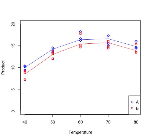
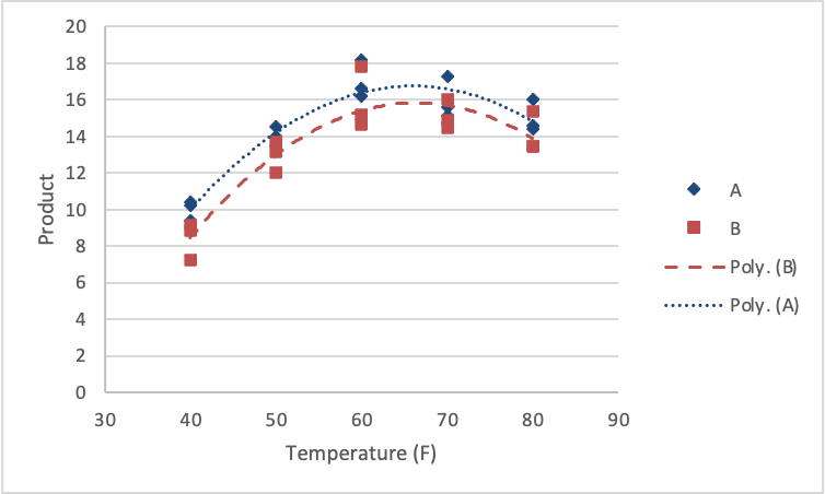
The linear and quadratic effects were significant in describing the trend in the response. Further, the linear and quadratic effects are the same for each of the reagent types (no interactions). A figure of the results would look as follows.
First, we load and attach the Quant Factor data.
setwd("~/path-to-folder/")
                    QuantFactor_data <- read.csv("QuantFactorData.csv",header=T)
                    attach(QuantFactor_data)
Next, we center and square the response variable and augment the dataset with the new variables.
temp_center = temp-60
                    temp_center2 = temp_center^2
                    new_data = data.frame(QuantFactor_data,temp_center,temp_center2)
                    detach(QuantFactor_data); attach(new_data)
We can then fit the ANCOVA using the recentered data and obtain the Type 1 ANOVA table (because polynomial models are built hierarchically). The output suggests that the regression coefficients of both the linear and quadratic terms are not statistically different for the treatment levels, i.e. the interactions are not significant, therefore those terms would be removed (sequentially) from the final model.
lm1 = lm(product ~ reagent + temp_center + temp_center2 + reagent:temp_center + reagent:temp_center2)
                    aov1 = aov(lm1)
                    summary(aov1)
Df Sum Sq Mean Sq F value Pr(>F)
reagent 1 9.24 9.24 8.948 0.00634 **
temp_center 1 97.60 97.60 94.519 8.50e-10 ***
temp_center2 1 88.83 88.83 86.028 2.09e-09 ***
reagent:temp_center 1 0.34 0.34 0.330 0.57075
reagent:temp_center2 1 0.07 0.07 0.065 0.80026
Residuals 24 24.78 1.03
---
Signif. codes: 0 ‘***’ 0.001 ‘**’ 0.01 ‘*’ 0.05 ‘.’ 0.1 ‘ ’ 1The regression curve for reagent A and reagent B can be plotted with the following commands.
data_subsetA = subset(new_data,reagent=="A")
                    data_subsetB = subset(new_data,reagent=="B")
                    lmA = lm(product ~ temp_center + temp_center2, data = data_subsetA)
                    lmB = lm(product ~ temp_center + temp_center2, data = data_subsetB)
                    plot(temp,product,ylim=c(0,20),xlab="Temperature", ylab="Product",pch=ifelse(reagent=="A",23,22), col=ifelse(reagent=="A","blue","red"), lwd=2)
                    lines(data_subsetA$temp,fitted(lmA), col = "blue")
                    lines(data_subsetB$temp,fitted(lmB), col = "red")
                    legend("bottomright",legend=c("A","B"),pch=c(23,22),col=c("blue","red"))