Here is the SAS code to run the ANOVA model for the hours of exercise for high school students example discussed in lesson 5.2:
data Nested_Example_data;
infile datalines delimiter=',';
input Region $ City $ ExHours;
datalines;
NE,NY,30
NE,NY,35
NE,Pittsburgh,18
NE,Pittsburgh,20
MW,Chicago,10
MW,Chicago,9
MW,Detroit,20
MW,Detroit,22
W,LA,18
W,LA,19
W,Seattle,4
W,Seattle,6
;
/*to run the nested ANOVA model*/
proc mixed data=Nested_Example_data method=type3;
class Region City;
model ExHours = Region City(Region);
store nested1;
run;
/*to obtain the resulting multiple comparison results*/
ods graphics on;
proc plm restore=nested1;
lsmeans Region / adjust=tukey plot=meanplot cl lines;
lsmeans City(Region) / adjust=tukey plot=meanplot cl lines;
run;
When we run this SAS program, here is the output that we are interested in:
| Type 3 Analysis of Variance | ||||||||
|---|---|---|---|---|---|---|---|---|
| Source | DF | Sum of Squares | Mean Square | Expected Mean Square | Error Term | Error DF | F Value | Pr > F |
| Region | 2 | 424.666667 | 212.333333 | Var(Residual)+Q(Region, City(Region)) | MS(Residual) | 6 | 65.33 | <.0001 |
| City(Region) | 3 | 496.750000 | 165.583333 | Var(Residual)+Q(City(Region)) | MS(Residual) | 6 | 50.95 | 0.0001 |
| Residual | 6 | 19.500000 | 3.250000 | Var(Residual) | ||||
| Type 3 Test of Fixed Effects | ||||
|---|---|---|---|---|
| Effect | Num DF | Den DF | F Value | Pr>F |
| Region | 2 | 6 | 65.33 | <.0001 |
| City(Region) | 3 | 6 | 50.95 | 0.0001 |
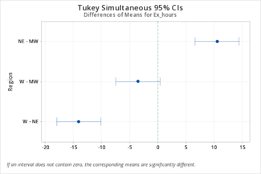
The p-values above indicate that both Region and City(Region) are statistically significant. The plots and charts below obtained from the Tukey option specify the means which are significantly different.
The exercise hours on average are statistically higher in the northeastern region compared to the midwest and the west, while the average exercise hours of these two regions are not significantly different.
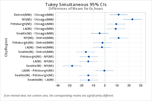
Also, the comparison of the means between cities indicates that the high schoolers in New York City exercise significantly more than the other cities in the study. The exercise levels are similar among Detroit, Pittsburgh, and LA, while the exercise levels of high schoolers in Chicago and Seattle are similar but significantly lower than all other cities in the study.
These grouping observations are further confirmed by the line plots below.
In Minitab, for the following (Nested Example Data):
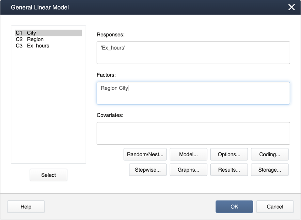
Stat > ANOVA > General Linear Model > Fit General Linear Model
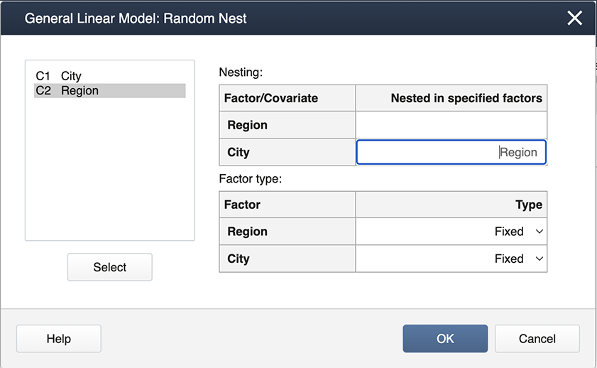
Enter the factors, 'Region' and 'City' in the Factors box, then click on Random/Nest...Here is where we specify the nested effect of City in Region.
The output is shown below.
Factor Information
General Linear Model: response versus School, Instructor
| Factor | Type | Levels | Values |
|---|---|---|---|
| Region | Fixed | 3 | MW, NE, W |
| City(Region) | Fixed | 6 |
Chicago(MW), Detroit(MW), NY (NE), Pittsburgh(NE), LA(W). Seattle(W) |
Analysis of Variance
| Source | D | Adj SS | Adj MS | F-Value | P-Value |
|---|---|---|---|---|---|
| Region | 2 | 424.67 | 212.333 | 65.33 | 0.000 |
| City(Region) | 3 | 496.75 | 165.583 | 50.95 | 0.000 |
| Error | 6 | 19.50 | 3.250 | ||
| Total | 11 | 940.92 |
Model Summary
| S | R-sq | R-sq(adj) | R-sq(pred) |
|---|---|---|---|
| 1.80278 | 97.93% | 96.20% | 91.71% |
Following the ANOVA run, you can generate the mean comparisons by
Stat > ANOVA > General Linear Model > Comparisons
Then specify “Region” and “City(Region)” for the comparisons by checking the boxes.
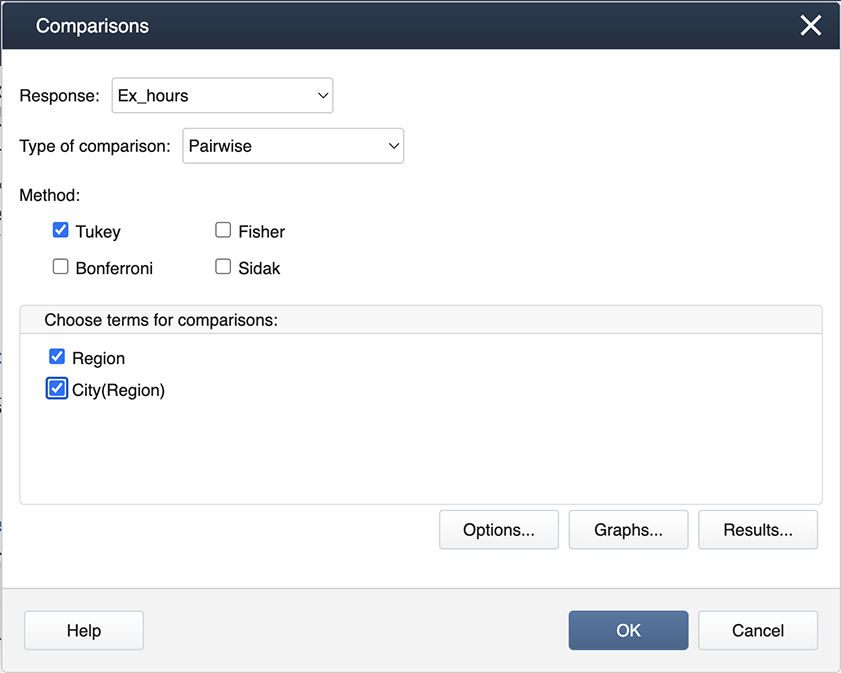
Then choose Graphs to get the following dialog box, where ‘Interval plot for the difference of means’ should be checked.
The outputs are as follows.
Tukey Pairwise Comparisons: Region
Grouping Information Using Tukey Method and 95% Confidence
| Region | N | Mean | Grouping |
|---|---|---|---|
| NE | 4 | 25.75 | A |
| MW | 4 | 15.25 | B |
| W | 4 | 11.75 | B |
Means that do not share a letter are significantly different.
Tukey Pairwise Comparisons: (City)Region
Grouping Information Using Tukey Method and 95% Confidence
| City(Region) | N | Mean | Grouping | |||
|---|---|---|---|---|---|---|
| NY(NE) | 2 | 32.5 | A | |||
| Detroit(MW) | 2 | 21.0 | B | |||
| Pittsburgh(NE) | 2 | 19.0 | B | |||
| LA(W) | 2 | 18.5 | B | |||
| Chicago(MW) | 2 | 9.5 | C | |||
| Seattle(W) | 2 | 5.0 | C | |||
Means that do not share a letter are significantly different.
Note: Nested models in R are a bit temperamental. If we run the model with nested (city) labels which are unique to each nesting factor (region), the resulting model will contain ALL interaction effects with NAs for those not included in the nested model. To avoid this, we can create a new variable in the dataset which labels the nested factors the same within each nesting factor. See below for an example.
First, load and attach the exercise hours data in R. We create a city code for each of the cities within each region. The data is below printed to illustrate the new variable.
setwd("~/path-to-folder/")
exhours_data<-read.table("exhours_data.txt",header=T,sep ="\t")
exhours_data$CityCode = as.factor(rep(c(1,1,2,2),3))
attach(exhours_data)
exhours_data
   Region       City Ex_hours CityCode
1      NE         NY       30        1
2      NE         NY       35        1
3      NE Pittsburgh       18        2
4      NE Pittsburgh       20        2
5      MW    Chicago       10        1
6      MW    Chicago        9        1
7      MW    Detroit       20        2
8      MW    Detroit       22        2
9       W         LA       18        1
10      W         LA       19        1
11      W    Seattle        4        2
12      W    Seattle        6        2
We run the model with the coded nested variable and obtain the ANOVA table.
options(contrasts=c("contr.sum","contr.poly"))
lm1 = lm(Ex_hours ~ Region/CityCode) # equivalent to lm1 = lm(Ex_hours ~ Region + Region:CityCode)
aov3 = car::Anova(lm1, type=3)
aov3
Anova Table (Type III tests)

Response: Ex_hours
                Sum Sq Df  F value    Pr(>F)
(Intercept)     3710.1  1 1141.564 4.475e-08 ***
Region           424.7  2   65.333 8.462e-05 ***
Region:CityCode  496.7  3   50.949 0.0001162 ***
Residuals         19.5  6
---
Signif. codes:  0 ‘***’ 0.001 ‘**’ 0.01 ‘*’ 0.05 ‘.’ 0.1 ‘ ’ 1
We can obtain the Tukey comparison of the regions as follows.
aov1 = aov(lm1)
tpairs_Region = TukeyHSD(aov1,"Region")
tpairs_Region
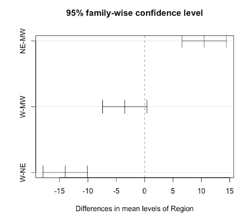
plot(tpairs_Region)
Tukey multiple comparisons of means
95% family-wise confidence level
Fit: aov(formula = lm1)
$Region
       diff        lwr         upr     p adj
NE-MW  10.5   6.588702  14.4112978 0.0004243
W-MW   -3.5  -7.411298   0.4112978 0.0747598
W-NE  -14.0 -17.911298 -10.0887022 0.0000836
If we were to use lm1 to obtain the Tukey comparison of the cities, our results would be labeled with the city codes, which is not easily interpreted. To obtain results with the city names, we will rerun the model with the variable City and omit the NAs from the Tukey results before displaying them.
lm2 = lm(Ex_hours ~ Region/City)
aov2 = aov(lm2)
tpairs_City = TukeyHSD(aov2,"Region:City")
tpairs_City$`Region:City` = na.omit(tpairs_City$`Region:City`)
tpairs_City
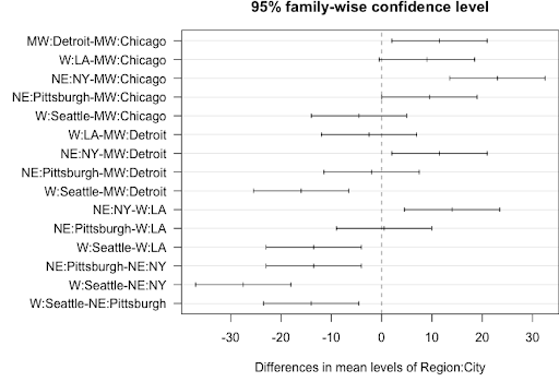
par(las = 1, mar=c(4.5,12,2,0)); plot(tpairs_City)
Tukey multiple comparisons of means
95% family-wise confidence level
Fit: aov(formula = lm2)
$`Region:City`
                          diff          lwr        upr     p adj
MW:Detroit-MW:Chicago     11.5   2.03420257  20.965797 0.0198222
W:LA-MW:Chicago            9.0  -0.46579743  18.465797 0.0626471
NE:NY-MW:Chicago          23.0  13.53420257  32.465797 0.0004610
NE:Pittsburgh-MW:Chicago   9.5   0.03420257  18.965797 0.0491884
W:Seattle-MW:Chicago      -4.5 -13.96579743   4.965797 0.5867601
W:LA-MW:Detroit           -2.5 -11.96579743   6.965797 0.9752059
NE:NY-MW:Detroit          11.5   2.03420257  20.965797 0.0198222
NE:Pittsburgh-MW:Detroit  -2.0 -11.46579743   7.465797 0.9960158
W:Seattle-MW:Detroit     -16.0 -25.46579743  -6.534203 0.0035460
NE:NY-W:LA                14.0   4.53420257  23.465797 0.0072412
NE:Pittsburgh-W:LA         0.5  -8.96579743   9.965797 1.0000000
W:Seattle-W:LA           -13.5 -22.96579743  -4.034203 0.0087623
NE:Pittsburgh-NE:NY      -13.5 -22.96579743  -4.034203 0.0087623
W:Seattle-NE:NY          -27.5 -36.96579743 -18.034203 0.0001762
W:Seattle-NE:Pittsburgh  -14.0 -23.46579743  -4.534203 0.0072412