To illustrate the role the covariate has in the ANCOVA, let’s look at a hypothetical situation wherein investigators are comparing the salaries of male vs. female college graduates. A random sample of 5 individuals for each gender is compiled, and a simple one-way ANOVA is performed:
| Males | Females |
|---|---|
| 78 | 80 |
| 43 | 50 |
| 103 | 30 |
| 48 | 20 |
| 80 | 60 |
\(H_0 \colon \mu_{\text{ Males}}=\mu_{\text{ Females}}\)
SAS coding for the one-way ANOVA:
data ancova_example;
input gender $ salary;
datalines;
m 78
m 43
m 103
m 48
m 80
f 80
f 50
f 30
f 20
f 60
;
proc mixed data=ancova_example method=type3;
class gender;
model salary=gender;
run;
Here is the output we get:
| Type 3 Tests of Fixed Effects | ||||
|---|---|---|---|---|
| Effect | Num DF | Den DF | F Value | Pr > F |
| gender | 1 | 8 | 2.11 | 0.1840 |
To perform a one-way ANOVA test in Minitab, you can first open the data (ANCOVA Example Minitab Data) and then select Stat > ANOVA > One Way…
In the pop-up window that appears, select salary as the Response and gender as the Factor.
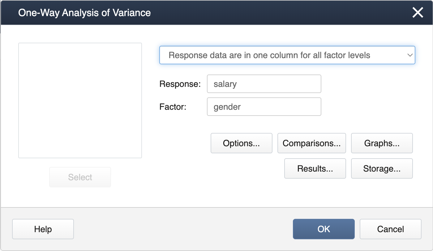
Click OK, and the output is as follows.
Analysis of Variance
| Source | DF | SS | SS | F-Value | P-Value |
|---|---|---|---|---|---|
| gender | 1 | 1254 | 1254 | 2.11 | 0.184 |
| Error | 8 | 4745 | 593 | ||
| Total | 9 | 6000 |
Model Summary
| S | R-sq | R-sq(adj) | R-sq(pred) |
|---|---|---|---|
| 24.3547 | 20.91% | 11.02% | 0.00% |
First, we can input the data manually for such a small dataset.
gender = c(rep("m",5),rep("f",5))
salary = c(78,43,103,48,80,80,50,30,20,60)
We then apply a simple one-way ANOVA and display the ANOVA table.
Anova Table (Type III tests)

Response: salary
             Sum Sq Df  F value     Pr(>F)
(Intercept) 35046.4  1 59.08522 5.8151e-05 ***
gender       1254.4  1  2.11481    0.18396
Residuals    4745.2  8
---
Signif. codes:  0 ‘***’ 0.001 ‘**’ 0.01 ‘*’ 0.05 ‘.’ 0.1 ‘ ’ 1