Exercise 1 Section
Three teaching methods were to be compared to teach computer science in high schools. Nine different schools were chosen randomly, and each teaching method was assigned to 3 randomly chosen schools, so each school implemented only one teaching method. The response used to compare the 3 teaching methods was the average score for each high school.
    data Lesson6_ex1;
    input mtd school score semester $;
    datalines;
    1 1 68.11 Fall
    1 1 68.11 Fall
    1 1 68.21 Fall
    1 1 78.11 Spring
    1 1 78.11 Spring
    1 1 78.19 Spring
    1 2 59.21 Fall
    1 2 59.13 Fall
    1 2 59.11 Fall
    1 2 70.18 Spring
    1 2 70.62 Spring
    1 2 69.11 Spring
    1 3 64.11 Fall
    1 3 63.11 Fall
    1 3 63.24 Fall
    1 3 63.21 Spring
    1 3 64.11 Spring
    1 3 63.11 Spring
    2 1 84.11 Fall
    2 1 85.21 Fall
    2 1 85.15 Fall
    2 1 85.11 Spring
    2 1 83.11 Spring
    2 1 89.21 Spring
    2 2 93.11 Fall
    2 2 95.21 Fall
    2 2 96.11 Fall
    2 2 95.11 Spring
    2 2 97.27 Spring
    2 2 94.11 Spring
    2 3 90.11 Fall
    2 3 88.19 Fall
    2 3 89.21 Fall
    2 3 90.11 Spring
    2 3 90.11 Spring
    2 3 92.21 Spring
    3 1 74.2 Fall
    3 1 78.14 Fall
    3 1 74.12 Fall
    3 1 87.1 Spring
    3 1 88.2 Spring
    3 1 85.1 Spring
    3 2 74.1 Fall
    3 2 73.14 Fall
    3 2 76.21 Fall
    3 2 72.14 Spring
    3 2 76.21 Spring
    3 2 75.1 Spring
    3 3 80.12 Fall
    3 3 79.27 Fall
    3 3 81.15 Fall
    3 3 85.23 Spring
    3 3 86.14 Spring
    3 3 87.19 Spring
    ;
-
Using the information about the teaching method, school, and score only, the school administrators conducted a statistical analysis to determine if the teaching method had a significant impact on student scores. Perform a statistical analysis to confirm their conclusion.
-
If possible, perform any other additional statistical analyses.
-
To confirm their conclusion, a model with only the two factors, teaching method, and school was used, with school nested within the teaching method.
Input:
    data Lesson6_ex1;
    input mtd school score semester $;
    datalines;
    1 1 68.11 Fall
    1 1 68.11 Fall
    1 1 68.21 Fall
    1 1 78.11 Spring
    1 1 78.11 Spring
    1 1 78.19 Spring
    1 2 59.21 Fall
    1 2 59.13 Fall
    1 2 59.11 Fall
    1 2 70.18 Spring
    1 2 70.62 Spring
    1 2 69.11 Spring
    1 3 64.11 Fall
    1 3 63.11 Fall
    1 3 63.24 Fall
    1 3 63.21 Spring
    1 3 64.11 Spring
    1 3 63.11 Spring
    2 1 84.11 Fall
    2 1 85.21 Fall
    2 1 85.15 Fall
    2 1 85.11 Spring
    2 1 83.11 Spring
    2 1 89.21 Spring
    2 2 93.11 Fall
    2 2 95.21 Fall
    2 2 96.11 Fall
    2 2 95.11 Spring
    2 2 97.27 Spring
    2 2 94.11 Spring
    2 3 90.11 Fall
    2 3 88.19 Fall
    2 3 89.21 Fall
    2 3 90.11 Spring
    2 3 90.11 Spring
    2 3 92.21 Spring
    3 1 74.2 Fall
    3 1 78.14 Fall
    3 1 74.12 Fall
    3 1 87.1 Spring
    3 1 88.2 Spring
    3 1 85.1 Spring
    3 2 74.1 Fall
    3 2 73.14 Fall
    3 2 76.21 Fall
    3 2 72.14 Spring
    3 2 76.21 Spring
    3 2 75.1 Spring
    3 3 80.12 Fall
    3 3 79.27 Fall
    3 3 81.15 Fall
    3 3 85.23 Spring
    3 3 86.14 Spring
    3 3 87.19 Spring
    ;


proc mixed data=lesson6_ex1 method=type3;
class mtd school;
model score = mtd;
random school(mtd);
store results1;
run;

proc plm restore=results1;
lsmeans mtd / adjust=tukey plot=meanplot cl lines;
run;
Partial outputs:
Type 3 Analysis of Variance
Type 3 Analysis of Variance Source DF Sum of Squares Mean Square Expected Mean Square Error Term Error DF F Value Pr > F mtd 2 4811.400959 2405.700480 Var(Residual) + 6 Var(school(mtd)) + Q(mtd) MS(school(mtd)) 6 16.50 0.0036 school(mtd) 6 875.059744 145.843291 Var(Residual) + 6 Var(school(mtd)) MS(Residual) 45 10.13 <.0001 Residual 45 647.972350 14.399386 Var(Residual) . . . . The p-value of 0.0036 indicates that the scores vary significantly among the 3 teaching methods, confirming the school administrators’ conclusion. As the teaching method was significant, the Tukey procedure was conducted to determine the significantly different pairs among the 3 teaching methods. The results of the Tukey procedure shown below indicate that the mean scores of teaching methods 2 and 3 are not statistically significant and that the teaching method 1 mean score is statistically lower than the mean scores of the other two.


- Using the additional code shown below, an ANOVA was conducted including semester also as a fixed effect.
proc mixed data=lesson6_ex1 method=type3;
class mtd school semester ;
model score = mtd semester mtd*semester;
random  school(mtd) semester*school(mtd);
store results2;
run;

proc plm restore= results2;
lsmeans mtd semester / adjust=tukey plot=meanplot cl lines;
run;
Type 3 Analysis of Variance
Type 3 Analysis of Variance Source DF Sum of Squares Mean Square Expected Mean Square Error Term Error DF F Value Pr > F mtd 2 4811.400959 2405.700480 Var(Residual) + 3 Var(school*semester(mtd)) + 6 Var(school(mtd)) + Q(mtd,mtd*semester) MS(school(mtd)) 6 16.50 0.0036 semester 1 286.166224 286.166224 Var(Residual) + 3 Var(school*semester(mtd)) + Q(semester,mtd*semester) MS(school*semester(mtd)) 6 8.34 0.0278 mtd*semester 2 85.703404 42.851702 Var(Residual) + 3 Var(school*semester(mtd)) + Q(mtd*semester) MS(school*semester(mtd)) 6 1.25 0.3520 school(mtd) 6 875.059744 145.843291 Var(Residual) + 3 Var(school*semester(mtd)) + 6 Var(school(mtd)) MS(school*semester(mtd)) 6 4.25 0.0508 school*semester(mtd) 6 205.848456 34.308076 Var(Residual) + 3 Var(school*semester(mtd)) MS(Residual) 36 17.58 <.0001 Residual 36 70.254267 1.951507 Var(Residual) . . . . The p-values indicate both the main effects of the method and semester are statistically significant, but their interaction is not and can be removed from the model. The Tukey procedure indicates that the significances of paired comparisons for the teaching method remain the same as in the previous model. Between the two semesters, the scores are statistically higher in the spring compared to the fall.
Note! The output writes semester*school(mtd) as school*semester(mtd) due to SAS arranging effects in alphabetical order.semester Least Squares Means semester Estimate Standard Error DF t Value Pr > |t| Alpha Lower Upper Fall 76.6370 1.8265 6 41.96 <.0001 0.05 72.1677 81.1063 Spring 81.2411 1.8265 6 44.48 <.0001 0.05 76.7718 85.7104
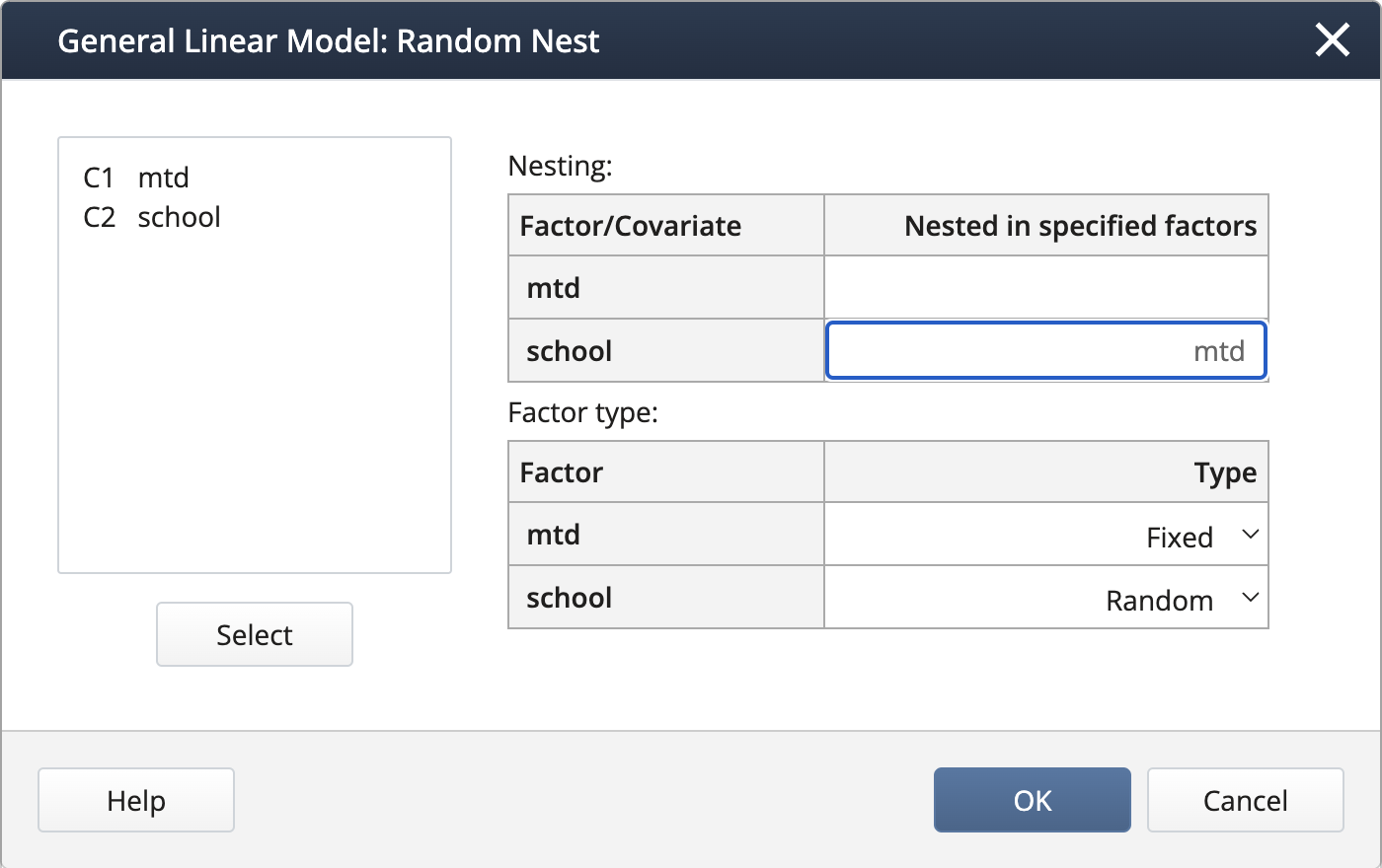
- In Stat > ANOVA > General Linear Model > Fit General Linear Model we complete the dialog box:

We create the nested term and specify the random effects under Random/Nest…:
Output:
Analysis of Variance
Source DF Adj SS Adj MS F-Value P-Value mtd 2 4811.4 2405.70 16.50 0.004 school(mtd) 6 875.1 145.84 10.13 0.000 Error 45 648.0 14.40 Total 53 6334.4 The p-value of 0.004 indicates that mtd is statistically significant. This implies that the mean score from all 3 teaching methods is not the same, confirming the school administrators’ claim. Note that in Minitab General Linear Model, the Tukey procedure or any other paired comparisons are not available.
-
In Stat > ANOVA > General Linear Model > Fit General Linear Model we complete the dialog box:

We create the nested term and specify the random effects under Random/Nest…:
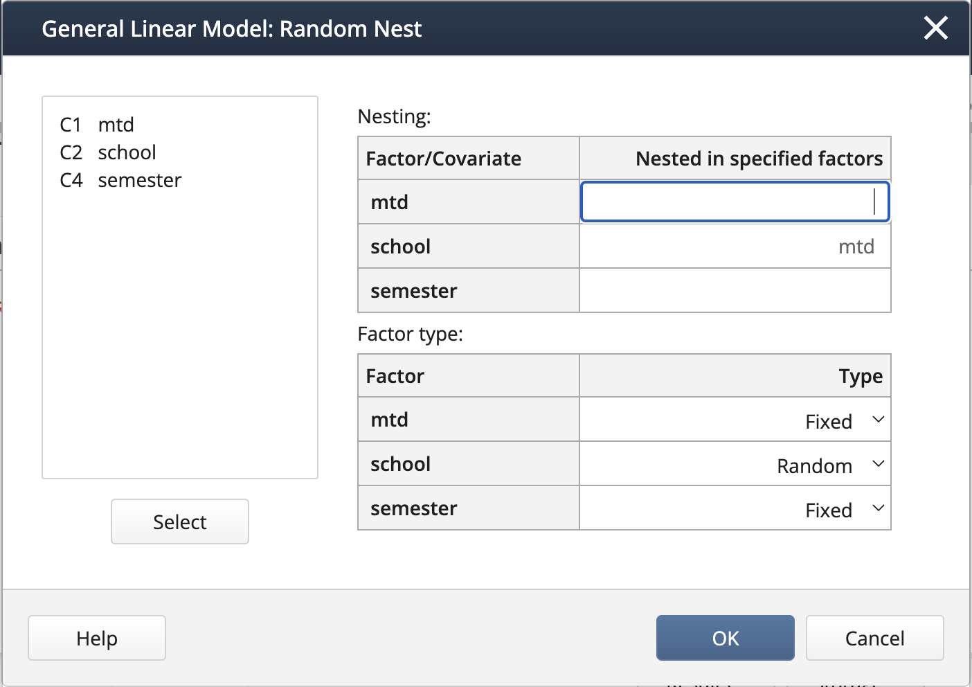
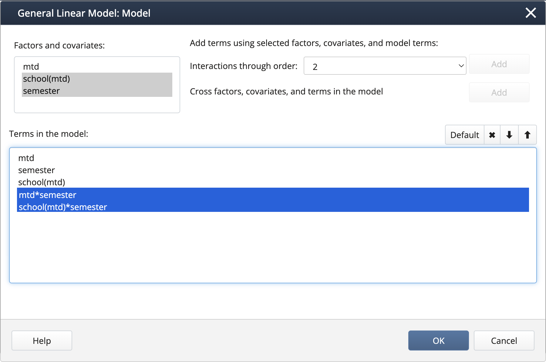
We can create interaction terms under Model… by selecting “mtd” and “semester” and clicking Add, then repeating for “school(mtd)” and “semester”.
Output:
Analysis of Variance
Source DF Adj SS Adj MS F-Value P-Value mtd 2 4811.40 2405.70 16.50 0.004 semester 1 286.17 286.17 8.34 0.028 school(mtd) 6 875.06 145.84 4.25 0.051 mtd*semester 2 85.70 42.85 1.25 0.352 school(mtd)*semester 6 205.85 34.31 17.58 0.000 Error 36 70.25 1.95 Total 53 6334.43 The p-values indicate that both main effects mtd and semester are statistically significant, but not their interaction.
Exercise 2 Section
| Type 3 Analysis of Variance | ||||||
|---|---|---|---|---|---|---|
| Source | DF | Sum of Squares | Mean Square | Expected Mean Square | F Value | Pr > F |
| Residual | 2 | 4811.400959 | 2405.700480 | Var(Residual) + 6 Var(A*B) + Q(A) | 11.38 | 0.0224 |
| 2 | 29.274959 | 14.637480 | Var(Residual) + 6 Var(A*B) + 18 Var(B) | 1.02 | 0.3700 | |
| 4 | 845.784785 | 211.446196 | Var(Residual)+ 6 Var(A*B) | 14.68 | <.0001 | |
| 45 | 647.972350 | 14.399386 | Var(Residual) | . | . | |
Use the ANOVA table above to answer the following.
- Name the fixed and random effects.
- Complete the Source column of the ANOVA table above.
- How many observations are included in this study?
- How many replicates are there?
- Write the model equation.
- Write the hypotheses that can be tested with the expression for the appropriate F statistic.
-
Name the fixed and random effects.
Fixed: A with 3 levels. In the EMS column, Q(A) reveals that A is fixed and the df indicates that it has 3 levels. Note that any factor that has a quadratic form associated with it is fixed and Q(A) is the quadratic form associated with A. This actually equals \(\sum_{i=1}^3\alpha_i^2\) where \(i = 1,2, 3\) are the treatment effects and is non-zero if the treatment means are significantly different.
Random: B is random as indicated by the presence of Var(B). The effect of factor B is studied by sampling 3 cases (see df value for B). A*B is random as any effect involving a random factor is random. The residual is also random as indicated by the presence of the Var(residual) in the EMS column.
-
Complete the Source column of the ANOVA table above.
Use the EMS column and start from the bottom row. The bottom-most has only Var(residual) and therefore the effect on the corresponding Source is residual. The next row up has Var(A*B) in the additional term indicating that the corresponding source is A*B, etc.
Type 3 Analysis of Variance Source DF Sum of Squares Mean Square Expected Mean Square F Value Pr > F A 2 4811.400959 2405.700480 Var(Residual) + 6 Var(A*B) + Q(A) 11.38 0.0224 B 2 29.274959 14.637480 Var(Residual) + 6 Var(A*B) + 18 Var(B) 1.02 0.3700 A*B 4 845.784785 211.446196 Var(Residual)+ 6 Var(A*B) 14.68 <.0001 Residual 45 647.972350 14.399386 Var(Residual) . . -
How many observations are included in this study?
N-1 = 2 + 2 +4 + 45 = 53 so N = 54.
-
How many full replicates are there?
Let r = number of replicates. Then N = number of levels of A * number of levels of B * r = 3 * 3 * r. Therefore, \(9 \times r = 54\) which gives \(r=6\).
-
Write the model equation.
\(y_{ijk}=\mu+\alpha_i+\beta_j+(\alpha\beta)_{ij}+\epsilon_{ijk},\text{ }i,j=1,2,3\text{, and }k = 1,2,\dots,6\)
-
Write the hypotheses that can be tested with the F-statistic information.
Effect A
Hypotheses
\(H_0\colon\alpha_i=0 \text{ for all } i\) vs. \(H_a\colon\alpha_i \neq 0\), for at least one \(i=1,2,3\)
Note that \(\sum_{i=1}^3\alpha_i^2\) is the non-centrality parameter of the F statistics if \(H_a\) is true.F-statistic
\(\dfrac{2405.700480}{211.446196}=11.377\) with 2 and 4 degrees of freedom
Effect B
Hypotheses
\(H_0\colon\sigma_\beta^2=0\) vs. \(H_a\colon \sigma_\beta^2 > 0\)
F-statistic
\(\dfrac{14.63480}{211.446196}=0.0692\) with 2 and 4 degrees of freedom
Note that SAS uses the unrestricted model (mentioned in Section 6.5) which results in MSAB as the denominator of the F-test (verified by looking at the EMS expressions).
Effect A*B
Hypotheses
\(H_0\colon\sigma_{\alpha\beta}^2=0\) vs. \(H_a\colon\sigma_{\alpha\beta}^2> 0\)
F-statistic
\(\dfrac{211.446196}{14.399386}=14.685\) with 4 and 45 degrees of freedom