One-Way ANOVA
- Step 1: Import the data
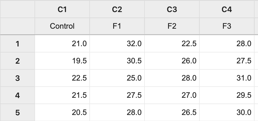
The data (Lesson1 Data) can be copied and pasted from a word processor into a worksheet in Minitab:
- Step 2: Run the ANOVA
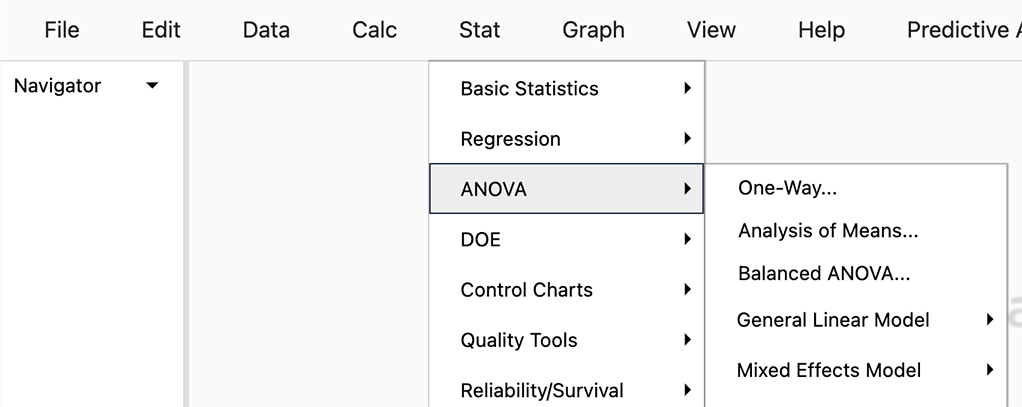
To run the ANOVA, we use the sequence of tool-bar tabs: Stat > ANOVA > One-way…
You then get the pop-up box seen below. Be sure to select from the drop-down in the upper right 'Response data are in a separate column for each factor level':
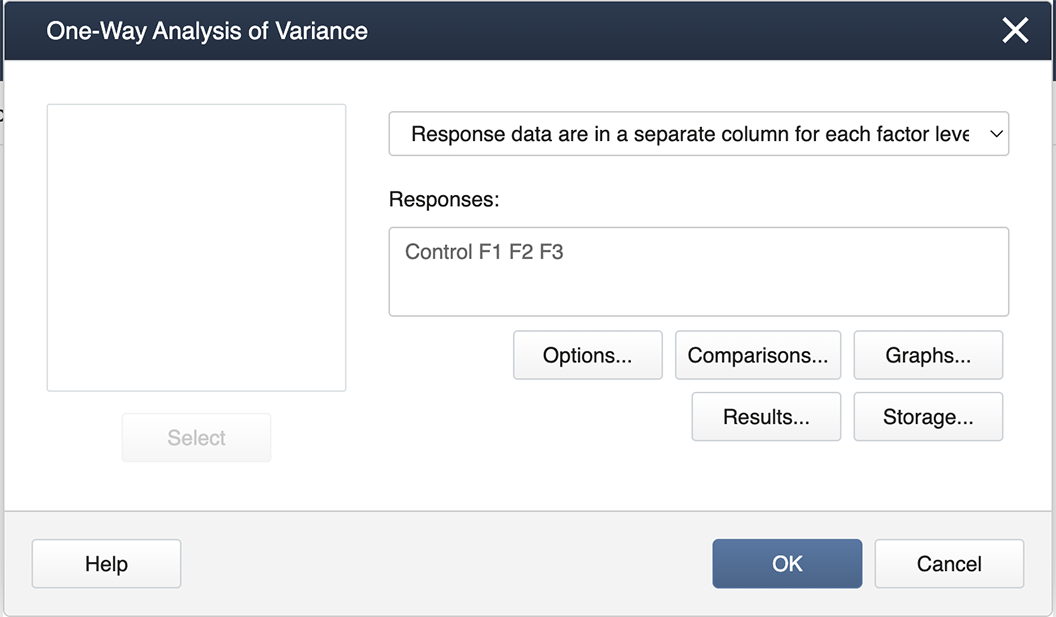
Then we double-click from the left-hand list of factor levels to the input box labeled ‘Responses’, and then click on the box labeled Comparisons.
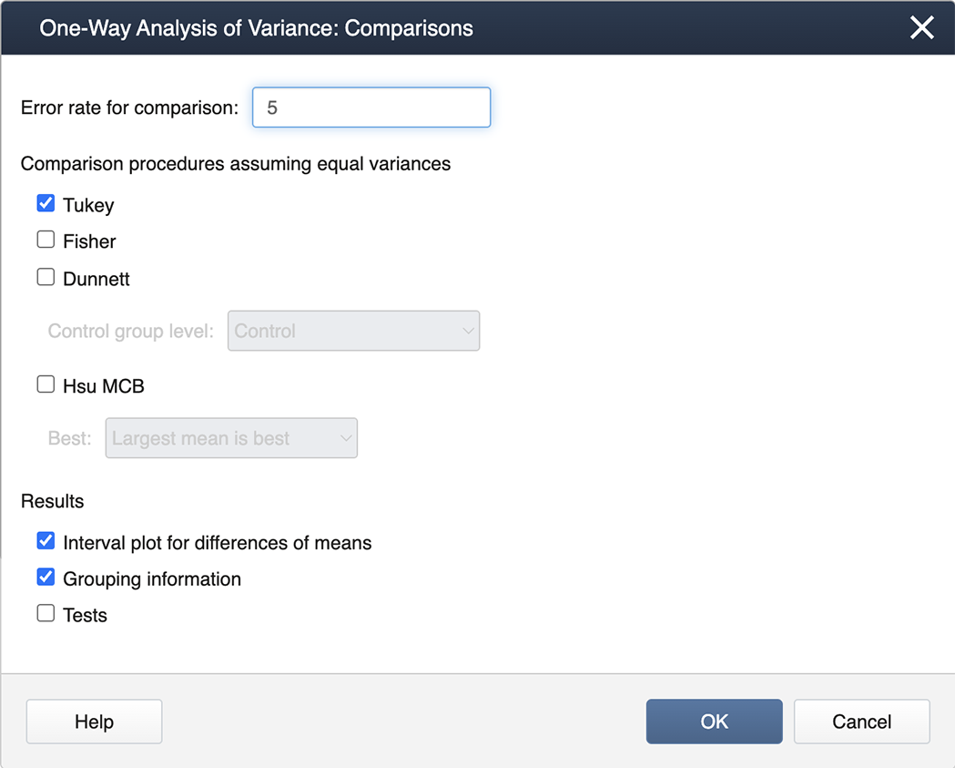
We check the box for Tukey and then exit by clicking on OK . To generate the Diagnostics, we then click on the box for Graphs and select the "Three in one" option:

You can now ‘back out' by clicking on OK in each nested panel.
- Step 3: Results
Now in the Session Window, we see the ANOVA table along with the results of the Tukey Mean Comparison:
One-Way ANOVA: Control, F1, F2, F3
Method
Null Hypothesis: All means are equal
Alternative Hypothesis: Not all means are equal
Significance Level: \(\alpha=0.05\)
Equal variances were assumed for the analysis.
Factor Information
Factor Levels Values Factor 4 Control, F1, F2, F3 Analysis of Variance
Source DF Adj SS Adj MS F-Value P-Value Factor 3 251.44 83.813 27.46 0.000 Error 20 61.03 3.052 Total 23 312.47 (Extracted from the output that follows from above.)
Grouping Information Using Tukey Method
N Mean Grouping F3 6 29.200 A F1 6 28.600 A B F2 6 25.867 B Control 6 21.000 C Means that do not share a letter are significantly different.
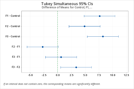
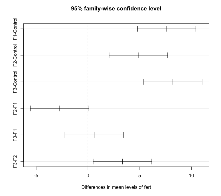
As can be seen, Minitab provides a difference in means plot, which can be conveniently used to identify the significantly different means by following the rule: if the confidence interval does not cross the vertical zero line, then the difference between the two associated means is statistically significant.
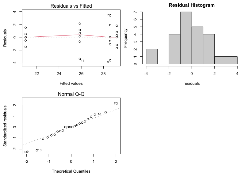
The diagnostic (residual) plots, as we asked for them, are in one figure:
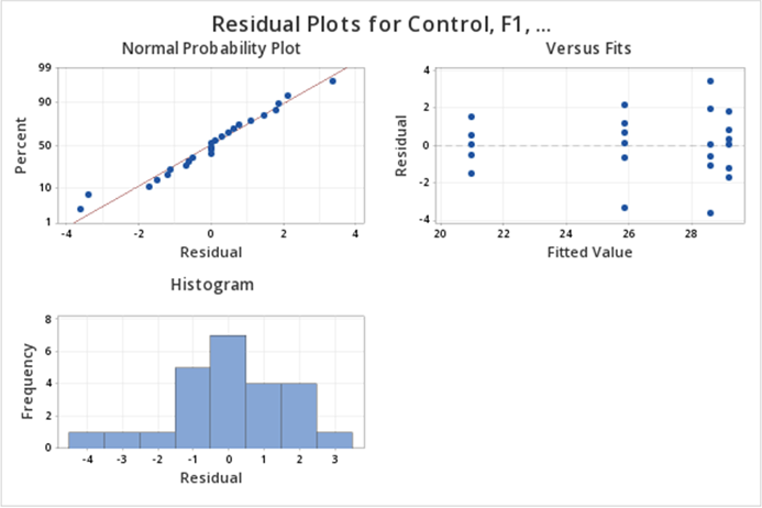
Note that the Normal Probability plot is reversed (i.e, the axes are switched) compared to the SAS output. Assessing straight line adherence is the same, and the residual analysis provided is comparable to SAS output.
First, load the greenhouse data in R. Note the greenhouse data are in separate columns.
setwd("~/path-to-folder/")
greenhouse_data<-read.table("greenhouse_data.txt",header=T)
We put our data in a stacked format; the first column has the response variable (height) and the second column has the treatment levels (fert). We can then attach the stacked dataset.
my_data<-stack(greenhouse_data)
colnames(my_data)<-c("height","fert")
attach(my_data)
To calculate the overall mean, standard deviation, and standard error we can use the following commands:
overall_mean<-mean(height)
overall_mean
[1] 26.16667
overall_sd<-sd(height)
overall_sd
[1] 3.685892
overall_standard_error<-overall_sd/sqrt(length(height))
overall_standard_error
[1] 0.7523795
Next, we calculate the mean, standard deviation, and standard error for each group.
aggregate(height~fert, FUN=mean)
     fert   height
1 Control 21.00000
2      F1 28.60000
3      F2 25.86667
4      F3 29.20000
aggregate(height~fert, FUN=sd)
     fert   height
1 Control 1.000000
2      F1 2.437212
3      F2 1.899123
4      F3 1.288410
std_error_fn = function(x){ sd(x)/sqrt(length(x)) }
aggregate(height~fert, FUN=std_error_fn)
     fert    height
1 Control 0.4082483
2      F1 0.9949874
3      F2 0.7753136
4      F3 0.5259911
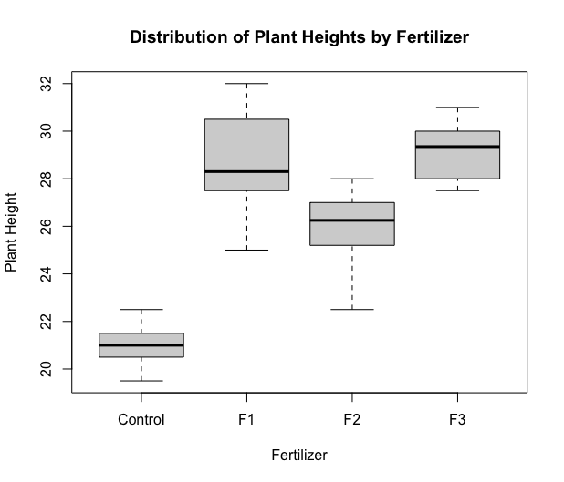
Next, we produce a boxplot.
boxplot(height~fert,xlab="Fertilizer",ylab="Plant Height",
         main="Distribution of Plant Heights by Fertilizer")
Next, we run the ANOVA model. The most commonly used function for ANOVA in R is aov. However, this function implements a sequential sum of squares (Type 1). To implement Type 3 sum of squares, we utilize the Anova function within the car package. Type 3 hypotheses are only used with effects coding for categorical variables (which we will learn more about in later lessons). Therefore before we obtain the ANOVA table, we must change the coding options to contr.sum, i.e. effect coding.
options(contrasts=c("contr.sum","contr.poly"))

library(car)
lm1 = lm(height ~ fert, data=my_data)
aov3 = Anova(lm1, type=3)
aov3
Anova Table (Type III tests)

Response: height
             Sum Sq Df  F value    Pr(>F)
(Intercept) 16432.7  1 5384.817 < 2.2e-16 ***
fert          251.4  3   27.465 2.712e-07 ***
Residuals      61.0 20
---
Signif. codes:  0 ‘***’ 0.001 ‘**’ 0.01 ‘*’ 0.05 ‘.’ 0.1 ‘ ’ 1
We can see the sum of squares in the first column, the degrees of freedom in the second column, the F-test statistic in the third column, and finally, we can see the p-value in the fourth column.
Note the output doesn't give the SSTotal. To find it, use the identity \(SSTotal=SSTreatment+SSResidual=251.44+61.03=312.47\). Similarly for the df associated with \(SSTotal\), we can add the df of \(SSTreatment\) and \(SSResidual\).
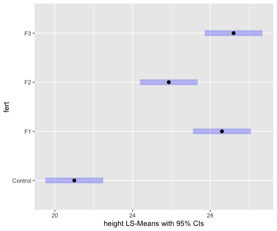
We can examine the LS means interval plot using the emmeans function (from the emmeans package) applied to the output of the aov function.
aov1 = aov(lm1) # equivalent to aov1 = aov(height ~ fert)
library(emmeans)
lsmeans = emmeans(aov1, ~fert)
plot(lsmeans, xlab="height LS-Means with 95% CIs")
To obtain the Tukey pairwise comparisons of means with a 95% family-wise confidence level we use the following commands:
tpairs = TukeyHSD(aov1)
tpairs
plot(tpairs)
  Tukey multiple comparisons of means
    95% family-wise confidence level

Fit: aov(formula = lm1)

$fert
                diff        lwr         upr     p adj
F1-Control  7.600000  4.7770648 10.42293521 0.0000016
F2-Control  4.866667  2.0437315  7.68960188 0.0005509
F3-Control  8.200000  5.3770648 11.02293521 0.0000005
F2-F1      -2.733333 -5.5562685  0.08960188 0.0598655
F3-F1       0.600000 -2.2229352  3.42293521 0.9324380
F3-F2       3.333333  0.5103981  6.15626854 0.0171033
Alternatively, the emmeans package can be used as follows (output not shown):
lsmeans = emmeans(aov1, ~fert)
tpairs2 = pairs(lsmeans,adjust="Tukey")
tpairs2
plot(tpairs2)
Finally, we can produce diagnostic (residual) plots as follows:
par(mfcol=c(2,2),mar=c(4.5,4.5,2,0)) # produces plots in one figure
plot(aov1,1)
plot(aov1,2)
hist(aov1$residuals,main="Residual Histogram",xlab="residuals")