- Output
The first output of the ANOVA procedure (shown below) gives useful details about the model.
ANOVA of Greenhouse Data
The Mixed Procedure
Model Information | |
|---|---|
Data Set | WORK.GREENHOUSE |
Dependent Variable | Height |
Covariance Structure | Diagonal |
Estimation Method | Type 3 |
Residual Variance Method | Factor |
Fixed Effects SE Method | Model-Based |
Degrees of Freedom Method | Residual |
Class Level Information | ||
|---|---|---|
Class | Levels | Values |
fert | 4 | Control F1 F2 F3 |
Dimensions | |
|---|---|
Covariance Parameters | 1 |
Columns in X | 5 |
Columns in Z | 0 |
Subjects | 0 |
Max Obs Per Subject | 24 |
The output below titled ‘Type 3 Analysis of Variance’ is similar to the ANOVA table we are already familiar with. Note that it does not include the Total SS, however it can be computed as the sum of all SS values in the table.
Type 3 Analysis of Variance | ||||||||
|---|---|---|---|---|---|---|---|---|
Sources | DF | Sum of Squares | Mean Square | Expected Mean Square | Error Term | Error DF | F Value | Pr > F |
fert | 3 | 251.440000 | 83.813333 | Var(Residual)+Q(fert) | MS(Residual) | 20 | 27.46 | <.0001 |
Residual | 20 | 61.033333 | 3.051667 | Var(Residual) | ||||
Covariance Parameter Estimates | |
|---|---|
Cov Parm | Estimate |
Residual | 3.0517 |
Fit Statistics | |
|---|---|
-2 Res Log Likelihood | 86.2 |
AIC (smaller is better) | 88.2 |
AICC (smaller is better) | 88.5 |
BIC (smaller is better) | 89.2 |
Type 3 Tests of Fixed Effects | ||||
|---|---|---|---|---|
Effect | Num DF | Den DF | F Value | Pr > F |
fert | 3 | 20 | 27.46 | <.0001 |
The output above titled “Type 3 Tests of Fixed Effects” will display the \(F_{\text{calculated}}\) and p-value for the test of any variables that are specified in the model statement. Additional information can also be requested. For example, the method = type 3 option will include the Expected Mean Squares (EMS) for each source, which will be useful in Lesson 6.
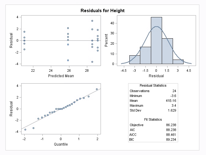
The mixed procedure also produces the following diagnostic plots:

The following display is a result of the LSmeans statement in the PLM procedure which was included in the programming code.
fert Least Squares Means | ||||||||
|---|---|---|---|---|---|---|---|---|
fert | Estimate | Standard Error | DF | t Value | Pr > |t| | Alpha | Lower | Upper |
Control | 21.0000 | 0.7132 | 20 | 29.45 | <.0001 | 0.05 | 19.5124 | 22.4876 |
F1 | 28.6000 | 0.7132 | 20 | 40.10 | <.0001 | 0.05 | 27.1124 | 30.0876 |
F2 | 25.8667 | 0.7132 | 20 | 36.27 | <.0001 | 0.05 | 24.3790 | 27.3543 |
F3 | 29.2000 | 0.7132 | 20 | 40.94 | <.001 | 0.05 | 27.7124 | 30.6876 |
In the "Least Squares Means" table above, note that the t-value and Pr >|t| are testing null hypotheses that each group mean= 0. (These tests usually do not provide any useful information). The Lower and Upper values are the 95% confidence limits for the group means. Note also that the least square means are the same as the original arithmetic means that were generated in the Summary procedure in Section 3.3 because all 4 groups have the same sample sizes. With unequal sample sizes or if there is a covariate present, the least square means can differ from the original sample means.
Next, the Plot= mean plot option in the LSmeans statement yields a mean plot and also a diffogram, shown below. The confidence intervals in the mean plot are commonly used to identify the significantly different treatment levels or groups. If two confidence intervals do not overlap, then the difference between the two associated means is statistically significant, which is a valid conclusion. However, if they overlap, it may be the case that the difference might still be significant. Consequently, conclusions made based on the visual inspection of the mean plot may not match with those arrived at using the table of ‘Difference of Least Square Means’, another output of the Tukey procedure, and is displayed below.
Notice this output is different from the previous table because it displays the results of each pairwise comparison. For example, the first row shows the comparison between the control and F1. The interpretation of these results is similar to any other confidence interval for the difference in two means - if the confidence interval does not contain zero, then the difference between the two associated means is statistically significant.
Differences of fert Least Squares Means Adjustment for Multiple Comparisons: Tukey | ||||||||||||
|---|---|---|---|---|---|---|---|---|---|---|---|---|
fert | _fert | Estimate | Standard Error | DF | t Value | Pr > |t| | Adj P | Alpha | Lower | Upper | Adj Lower | Adj Upper |
Control | F1 | -7.6000 | 1.0086 | 20 | -7.54 | <.0001 | <.0001 | 0.05 | -9.7038 | -5.4962 | -10.4229 | -4.7771 |
Control | F2 | -4.8667 | 1.0086 | 20 | -4.83 | 0.0001 | 0.0006 | 0.05 | -6.9705 | -2.7628 | -7.6896 | -2.0438 |
Control | F3 | -8.2000 | 1.0086 | 20 | -8.13 | <.0001 | <.0001 | 0.05 | -10.3038 | -6.0962 | -11.0229 | -5.3771 |
F1 | F2 | 2.7333 | 1.0086 | 20 | 2.71 | 0.0135 | 0.0599 | 0.05 | 0.6295 | 4.8372 | -0.08957 | 5.5562 |
F1 | F3 | -0.6000 | 1.0086 | 20 | -0.59 | 0.5586 | 0.9324 | 0.05 | -2.7038 | 1.5038 | -3.4229 | 2.2229 |
F2 | F3 | -3.3333 | 1.0086 | 20 | -3.30 | 0.0035 | .0171 | 0.05 | -5.4372 | -1.2295 | -6.1562 | -0.5104 |
This discrepancy between the mean plot and the ‘Difference of Least Square Means’ results occurs because the testing is done in terms of the difference of two means, using the standard error of the difference of the two-sample means, but the confidence intervals of the mean plot are computed for the individual means which are in terms of the standard error of individual sample means. Consistent results can be achieved by using the diffogram as discussed below or the confidence intervals displayed in the ‘difference in mean plot’ available in SAS 14, but not included here.
The diffogram has two useful features. It allows one to identify the significant mean pairs and also gives estimates of the individual means. The diagonal line shown in the diffogram is used as a reference line. Each group (or factor level) is marked on the horizontal and vertical axes and has vertical and horizontal reference lines with their intersection point falling on the diagonal reference line. The x or the y coordinates of this intersection point which are equal is the sample mean of that group. For example, the sample mean for the Control group is about 21, which matches with the estimate provided in the ‘Least Squares Means’ table displayed above. Furthermore, each slanted line represents a mean pair. Start with any group label from the horizontal axis and run your cursor up along the associated vertical line until it meets a slanted line, and then go across the intersecting horizontal line to identify the other group (or factor level). For example, the lowermost solid line (colored blue) represents the Control and F2. As stated at the bottom of the chart, the solid (or blue) lines indicate significant pairs, and the broken (or red) lines correspond to the non-significant pairs. Furthermore, a line corresponding to a nonsignificant pair will cross the diagonal reference line.
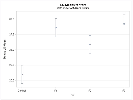
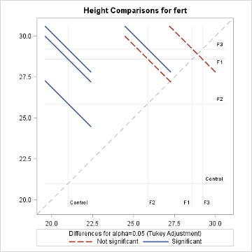
The non-overlapping confidence intervals in the mean plot above indicate that the average plant height due to control is significantly different from those of the other 3 fertilizer levels and that the F2 fertilizer type yields a statistically different average plant height from F3. The diffogram also delivers the same conclusions and so, in this example, conclusions are not contradictory. In general, the diffogram always provides the same conclusions as derived from the confidence intervals of difference of least-square means shown in the ‘Difference of Least Square Means’ table, but the conclusions based on the mean plot may differ.
There are two contrasts of interest: contrast to compare the control and F3 with F1 and F2 (i.e. \(\mu_{control}-\mu_{F_1}-\mu_{F_2}+\mu_{F_3}\)) and the contrast to compare control and F2 with F1 (i.e. \(\mu_{control}-2\mu_{F_1}+\mu_{F_2}\)). Since we are testing for two contrasts, we should adjust for multiple comparisons. We use Bonferroni adjustment. In SAS, we can use the estimate command under proc plm to make these computations.
In general, the estimate command estimates linear combinations of model parameters and performs t-tests on them. Contrasts are linear combinations that satisfy a special condition. We will discuss the model parameters in Lesson 4.
Estimates | ||||||
|---|---|---|---|---|---|---|
Label | Estimate | Standard Error | DF | t Value | Pr > |t| | Adj P |
Compare control + F3 with F1 and F2 | -4.2667 | 1.4263 | 20 | -2.99 | 0.0072 | 0.0144 |
Compare control + F2 with F1 | -10.3333 | 1.7469 | 20 | -5.92 | <.0001 | <.0001 |
SAS returns both unadjusted and adjusted p-values. Suppose we wanted to make the comparisons at 1% level. If we ignored the multiple comparisons (i.e. using unadjusted p-values), the both comparisons are statistically significant. However, if we consider the adjusted p-values, we will fail to reject the hypothesis corresponding to the first contrast at the 1% level.