A CRD for the greenhouse experiment is reasonable, provided the positions on the bench are equivalent. In reality, this is rarely the case. For example, some micro-environmental variation can be expected due to the glass wall on one end, and the open walkway at the other end of the bench.
A powerful alternative to the CRD is to restrict the randomization process to form blocks. In a block design, general blocks are formed such that the experimental units are expected to be homogeneous within a block and heterogeneous between blocks. The number of experimental units within a block is called its block size.
In a randomized complete block design (RCBD), each block size is the same and is equal to the number of treatments (i.e. factor levels or factor level combinations). Furthermore, each treatment will be randomly assigned to exactly one experimental unit within every block. So if we think of the greenhouse example, in a RCBD we will have 6 blocks, each with block size of 4 (the number of fertilizer levels).
To establish an RCBD for this data, the assignments of fertilizer levels to the experimental units (the potted plants) have to be done within each block separately. Examples of how to do this using statistical software will be detailed in the section below.
It is important to mention that blocks are usually (but not always) treated as random effects as they typically represent the population of all possible blocks. In other words, the mean comparison among specific blocks is not of interest. However, the variation between blocks must be incorporated into the model. In a RCBD, the variation between blocks is partitioned out of the MSE of the CRD, resulting in a smaller MSE for testing hypotheses about the treatments.
The statistical model corresponding to the RCBD is similar to the two-factor studies with one observation per cell (i.e. we assume the two factors do not interact).
Here is Dr. Shumway stepping through this experimental design in the greenhouse.
We will consider the greenhouse experiment with one factor of interest (Fertilizer). We also have the identifications for the blocks. In this example, we consider Fertilizer as a fixed effect (as we are only interested in comparing the 4 fertilizers we chose for the study) and Block as a random effect.
Therefore the statistical model would be
\(Y_{ij} = \mu + \rho_i + \tau_j + \epsilon_{ij}\)
with \(i=1,2,\dots,6\) and \(j=1,2,3,4\). \(\rho_i\)s and \(\epsilon_{ij}\) are independent random variables such that \(\rho_i \sim \mathcal{N}\left(0, \sigma^2_{\rho}\right)\) and \(\epsilon_{ij}\sim \mathcal{N}\left(0, \sigma^2\right)\).
Using Technology Section
To obtain the block design in SAS, we can use the following code:
proc plan ordered ;
factors Block=6 Plant=4;
treatments Fertilizer=4 random;
output out=rcb block
cvals=('Block 1' 'Block 2' 'Block 3' 'Block 4' 'Block 5' 'Block 6');
run;
proc format;
value FertFmt
1 = "F1"
2 = "F2"
3 = "F3"
4 = "Con";
run;
proc print data=rcb;
format Fertilizer FertFmt.;
run;
The output we obtain would be as follows:
| Obs | Block | Plant | Fertilizer |
|---|---|---|---|
| 1 | Block 1 | 1 | F3 |
| 2 | Block 1 | 2 | F2 |
| 3 | Block 1 | 3 | Con |
| 4 | Block 1 | 4 | F1 |
| 5 | Block 2 | 1 | F1 |
| 6 | Block 2 | 2 | F3 |
| 7 | Block 2 | 3 | F2 |
| 8 | Block 2 | 4 | Con |
| 9 | Block 3 | 1 | F2 |
| 10 | Block 3 | 2 | Con |
| 11 | Block 3 | 3 | F3 |
| 12 | Block 3 | 4 | F1 |
| 13 | Block 4 | 1 | F2 |
| 14 | Block 4 | 2 | F3 |
| 15 | Block 4 | 3 | F1 |
| 16 | Block 4 | 4 | Con |
| 17 | Block 5 | 1 | F3 |
| 18 | Block 5 | 2 | F1 |
| 19 | Block 5 | 3 | Con |
| 20 | Block 5 | 4 | F2 |
| 21 | Block 6 | 1 | Con |
| 22 | Block 6 | 2 | F2 |
| 23 | Block 6 | 3 | F3 |
| 24 | Block 6 | 4 | F1 |
Once we collect the data for this experiment, we can use SAS to analyze the data and obtain the results.
Let us read the data into SAS and obtain the proc summary output.
data RCBD_oneway;
input block Fert $ Height;
datalines;
1      Control      19.5
2      Control      20.5
3      Control      21
4      Control      21
5      Control      21.5
6      Control      22.5
1      F1      25
2      F1      27.5
3      F1      28
4      F1      28.6
5      F1      30.5
6      F1      32
1      F2      22.5
2      F2      25.2
3      F2      26
4      F2      26.5
5      F2      27
6      F2      28
1      F3      27.5
2      F3      28
3      F3      29.2
4      F3      29.5
5      F3      30
6      F3      31
;
proc summary data=RCBD_oneway;
class block fert;
var height;
output out=output1 mean=mean stderr=se;
run;
proc print data=output1;
The proc summary output would be as follows. We see that the first line in the table with _TYPE_=0 identification is the estimated overall mean (i.e. \(\bar{y}_{\cdot\cdot}\)). The estimated treatment means (i.e. \(\bar{y}_{\cdot j}\)) are displayed with _TYPE_=1 identification and the estimated block means are displayed with _TYPE_=2 identification. Since we only have one observation per treatment within each block, we cannot estimate the standard error using the data.
| Obs | block | Fert | _TYPE_ | _FREQ_ | mean | se |
|---|---|---|---|---|---|---|
| 1 | . | 0 | 24 | 26.1667 | 0.75238 | |
| 2 | . | Control | 1 | 6 | 21.0000 | 0.40825 |
| 3 | . | F1 | 1 | 6 | 28.6000 | 0.99499 |
| 4 | . | F2 | 1 | 6 | 25.8667 | 0.77531 |
| 5 | . | F3 | 1 | 6 | 29.2000 | 0.52599 |
| 6 | 1 | 2 | 4 | 23.6250 | 1.71239 | |
| 7 | 2 | 2 | 4 | 25.3000 | 1.71221 | |
| 8 | 3 | 2 | 4 | 26.0500 | 1.80808 | |
| 9 | 4 | 2 | 4 | 26.4000 | 1.90657 | |
| 10 | 5 | 2 | 4 | 27.2500 | 2.06660 | |
| 11 | 6 | 2 | 4 | 28.3750 | 2.13478 | |
| 12 | 1 | Control | 3 | 1 | 19.5000 | . |
| 13 | 1 | F1 | 3 | 1 | 25.0000 | . |
| 14 | 1 | F2 | 3 | 1 | 22.5000 | . |
| 15 | 1 | F3 | 3 | 1 | 27.5000 | . |
| 16 | 2 | Control | 3 | 1 | 20.5000 | . |
| 17 | 2 | F1 | 3 | 1 | 27.5000 | . |
| 18 | 2 | F2 | 3 | 1 | 25.2000 | . |
| 19 | 2 | F3 | 3 | 1 | 28.0000 | . |
| 20 | 3 | Control | 3 | 1 | 21.0000 | . |
| 21 | 3 | F1 | 3 | 1 | 28.0000 | . |
| 22 | 3 | F2 | 3 | 1 | 26.0000 | . |
| 23 | 3 | F3 | 3 | 1 | 29.2000 | . |
| 24 | 4 | Control | 3 | 1 | 21.0000 | . |
| 25 | 4 | F1 | 3 | 1 | 28.6000 | . |
| 26 | 4 | F2 | 3 | 1 | 26.5000 | . |
| 27 | 4 | F3 | 3 | 1 | 29.5000 | . |
| 28 | 5 | Control | 3 | 1 | 21.5000 | . |
| 29 | 5 | F1 | 3 | 1 | 30.5000 | . |
| 30 | 5 | F2 | 3 | 1 | 27.0000 | . |
| 31 | 5 | F3 | 3 | 1 | 30.0000 | . |
| 32 | 6 | Control | 3 | 1 | 22.5000 | . |
| 33 | 6 | F1 | 3 | 1 | 32.0000 | . |
| 34 | 6 | F2 | 3 | 1 | 28.0000 | . |
| 35 | 6 | F3 | 3 | 1 | 31.0000 | . |
To run the model in SAS we can use the following code
/* RCBD */
proc mixed data=RCBD_oneway method=type3;
class block fert;
model height=fert;
random block;
run;
We obtain the ANOVA table below for the RCBD.
| Type 3 Analysis of Variance | ||||||||
|---|---|---|---|---|---|---|---|---|
| Source | DF | Sum of Squares | Mean Square | Expected Mean Square | Error Term | Error DF | F Value | Pr > F |
| Fert | 3 | 251.440000 | 83.813333 | Var(Residual) + Q(Fert) | MS(Residual) | 15 | 162.96 | <.0001 |
| block | 5 | 53.318333 | 10.663667 | Var(Residual) + 4 Var(block) | MS(Residual) | 15 | 20.73 | <.0001 |
| Residual | 15 | 7.715000 | 0.514333 | Var(Residual) | . | . | . | . |
For comparison, let us obtain the ANOVA table for the CRD for the same data. We use the following SAS commands:
/* CRD for comparison */
proc mixed data=RCBD_oneway method=type3;
class fert;
model height=fert;
run;
The CRD ANOVA table for our data would be as follows:
| Type 3 Analysis of Variance | ||||||||
|---|---|---|---|---|---|---|---|---|
| Source | DF | Sum of Squares | Mean Square | Expected Mean Square | Error Term | Error DF | F Value | Pr > F |
| Fert | 3 | 251.440000 | 83.813333 | Var(Residual) + Q(Fert) | MS(Residual) | 20 | 27.46 | <.0001 |
| Residual | 20 | 61.033333 | 3.051667 | Var(Residual) | . | . | . | . |
Comparing the two ANOVA tables, we see that the MSE in RCBD has decreased considerably in comparison to the CRD. This reduction in MSE can be viewed as the partition in SSE for the CRD (61.033) into SSBlock (53.32) + SSE (7.715). The potential reduction in SSE by blocking is offset to some degree by losing degrees of freedom for the blocks. But more often than not, is worth it in terms of the improvement in the calculated F-statistic. In our example, we observe that the F-statistic for the treatment has increased considerably for RCBD in comparison to CRD. It is reasonable to assume that the result from the RCBD is more valid than that from the CRD as the MSE value obtained after accounting for the block to block variability is a more accurate representation of the random error variance.
To obtain the design in Minitab, we do the following.
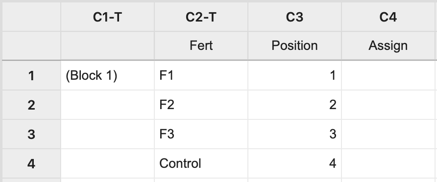
For Block 1, manually create two columns: one with each treatment level and the other with a position number 1 to n, where n is the block size (i.e. n = 4 in this example). The third column will store the assignment of fertilizer levels to the experimental units.
Next, select Calc > Sample from Columns > fill in the dialog box as seen below, and click OK.
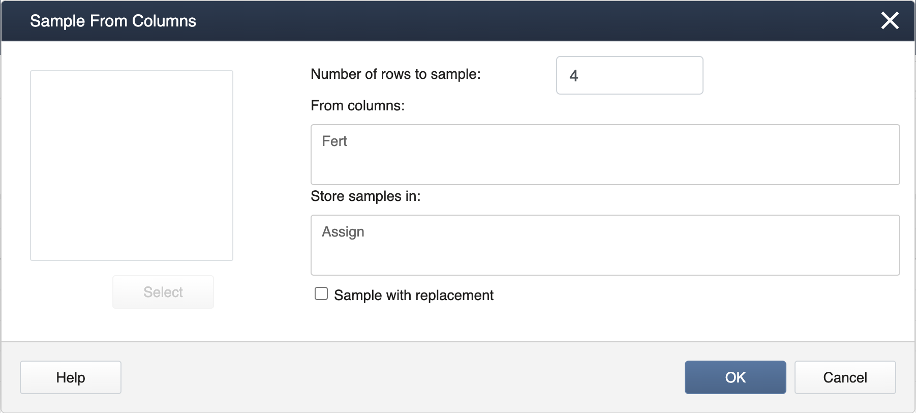
Here, the number of rows to be specified is our block size (and number of treatment levels) which yields a random assignment from Block 1.
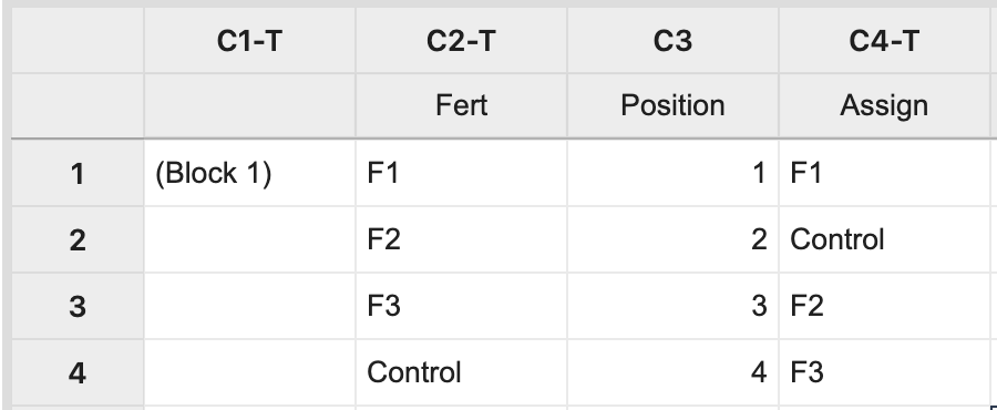
The same process should be repeated for the remaining blocks. The key element is that each treatment level or treatment combination appears in each block (forming complete blocks), and is assigned at random within each block.
To obtain the RCBD in R, we can use the blocks function from the blocksdesign package.
library(blocksdesign)
set.seed(1)
block_design = blocks(treatments = 4, replicates = 6, blocks = 6)$Design
We can then construct a data frame to view the design.
block = block_design[,1]
treatment = block_design[,3]
plant = rep(c(1:4),6)
data.frame(cbind(block,plant,treatment))
   block plant treatment
1      1     1         1
2      1     2         3
3      1     3         2
4      1     4         4
5      2     1         3
6      2     2         2
7      2     3         4
8      2     4         1
9      3     1         4
10     3     2         1
11     3     3         2
12     3     4         3
13     4     1         2
14     4     2         4
15     4     3         3
16     4     4         1
17     5     1         4
18     5     2         1
19     5     3         3
20     5     4         2
21     6     1         2
22     6     2         1
23     6     3         4
24     6     4         3