Recall the Randomized Complete Block Design (RCBD) we discussed in lesson 7. In RCBD, general blocks are formed such that the experimental units are expected to be homogenous within a block and heterogeneous between blocks.
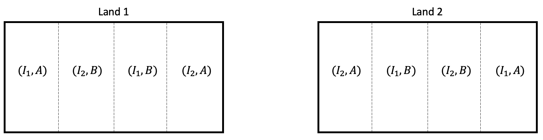
For example, suppose we are studying the effect of irrigation amount (\(I_1\) and \(I_2\)) and fertilizer type (\(A\) and \(B\)) on crop yield. We have 4 treatments in this experiment. Suppose we want to have at least 2 replicates and two large lands that can be used for the experiment. In RCBD, we can split each land into 4 fields and can apply the 4 treatments randomly to each field. Here lands are blocks and fields are the experimental units.
In this example, we have assumed that managing levels of irrigation and fertilizer require the same effort. Now suppose varying the level of irrigation is difficult on a small scale and it makes more sense to apply irrigation levels to larger areas of land.
In such situations, we can divide each land into two large fields (whole plots) and apply irrigation amounts to each field randomly. And then divide each of these large fields into smaller fields (subplots) and apply fertilizer randomly within the whole plots.
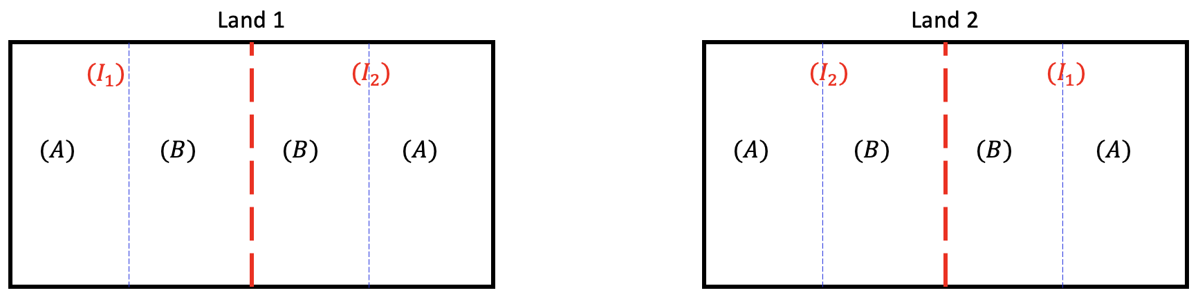
In this strategy, each land contains two whole plots and the irrigation amount is assigned to each whole plot randomly using RCBD (i.e. lands are treated as blocks, and the irrigation amount is assigned randomly within each block to the whole plots). Each whole plot contains two subplots and fertilizer type is assigned to each subplot using RCBD (i.e. whole plots are treated as blocks and fertilizer type is assigned randomly within each whole plot to the subplots).
When some factors are more difficult to vary than others at the level of experimental units, it is more efficient to assign the difficult-to-change factors to larger units (whole plots) and then apply the easier-to-change factor to smaller units (subplots). This is known as the split-plot design.
As an example, consider an experiment where fabric is dyed at 4 different temperatures for 3 different amounts of time. The differences in color saturation are of interest. If the experimenters desire 3 replications for each of the 12 temperature and time combinations (i.e. 12 treatments), a basic CRD or an RCBD (with a suitable blocking factor that would generate the replicates) will require as many as 36 attempts of testing.
Instead, the experiment can be modified as follows to reduce effort and time. Regarding dye tanks as blocks, the 3 tanks can be set to each of the 4 different temperature settings (sequentially and in random order). Then, for each tank and each temperature, the 3 fabrics are randomly selected to be taken out of the tank at the 3 different time intervals.
In this setting, temperatures are assigned randomly within each dye tank (i.e. tank is treated as a block), and within each temperature, the dying times are assigned randomly to the fabric. We have two RCBD sub-experiments: whole plot levels (temperatures) are assigned as RCBD within the tank and subplot levels (dying time) are assigned as RCBD within whole plot levels.
The data (Dye Time Data) were:
Tank Temperature | |||||
|---|---|---|---|---|---|
Rep | Dying Time (min) | 100 | 120 | 180 | 220 |
I | 20 | 15 | 32 | 56 | 58 |
40 | 33 | 47 | 62 | 65 | |
60 | 37 | 58 | 78 | 80 | |
II | 20 | 18 | 36 | 57 | 62 |
40 | 29 | 49 | 63 | 67 | |
60 | 32 | 55 | 75 | 79 | |
III | 20 | 16 | 33 | 54 | 57 |
40 | 27 | 43 | 67 | 63 | |
60 | 35 | 54 | 73 | 77 | |
It is important to notice that in a split-plot design, randomization is a two-stage process. Levels of one factor (say, factor A) are randomized over the whole plots within each block, and the levels of the other factor (say, factor B) are randomized over the subplots within each whole plot. This restriction in randomization results in two different error terms: one appropriate for comparisons at the whole plot level and one appropriate for comparisons at the subplot level.
The appropriate error for whole plot level in split-plot RCBD is \(\text{whole plot factor} \times \text{block}\) interaction. In other words, the analysis at the whole plot level is essentially a one-way ANOVA with blocking (i.e. one observation per block-treatment combination). From the perspective of the whole plot, the subplots are simply subsamples and it is reasonable to average them when testing the whole plot effects (i.e. factor A effects).
The subplot factor (i.e. factor B) is always compared within the whole plot factor.
Source | DF |
|---|---|
Blocks | \(r-1\) |
Factor \(A\) | \(a-1\) |
Blocks \(\times\) Factor \(A\) (Whole plot Error) | \((r-1)(a-1)\) |
Factor \(B\) | \(b-1\) |
\(A \times B\) | \((a-1)(b-1)\) |
Residual (Subplot Error) | a\((r-1)(b-1)\) |
Total | \(rab - 1\) |
The statistical model associated with the split-plot design with whole plots arranged as RCBD is
\(Y_{ijk} = \mu + \alpha_i + \gamma_k + (\alpha\gamma)_{ik} + \beta_j + (\alpha\beta)_{ij} + \epsilon_{ijk}\)
where \(\gamma_k\) for \(k=1,...,r\) are block effects, \(\alpha_i\) for \(i=1,...,a\) are factor A effects, and \(\beta_j\) for \(j=1,...,b\) are factor B effects.
Therefore, the ANOVA table for the example above would look like this:
Source | DF | Expected Mean Square | Error Term |
|---|---|---|---|
(Whole Plots) | |||
Blocks | 1 | Var(Residual) + 3Var(Blocks*A) + 12Var(Blocks) | MS(Blocks*A) |
A | 1 | Var(Residual) + 3Var(Blocks*A) + Q(A,A*B) | MS(Blocks*A) |
Blocks*A | 1 | Var(Residual) + 3Var(Blocks*A) | |
(Subplots) | |||
B | 1 | Var(Residual) + Q(B, A*B) | MS(Residual) |
A*B | 1 | Var(Residual) + Q(A*B) | MS(Residual) |
Residual | 2 | Var(Residual) |
Using Technology Section
In SAS, we could specify the model with the following statements:
proc mixed data=DyeTimeData method=type3;
                class tank temp time;
                model resp=temp time temp*time;
                random tank tank*temp;
                run;
This will generate the ANOVA table as below.
Type 3 Analysis of Variance | ||||||||
|---|---|---|---|---|---|---|---|---|
Source | DF | Sum of Squares | Mean Square | Expected Mean Square | Error Term | Error DF | F Value | Pr > F |
temp | 3 | 9762.333333 | 3254.111111 | Var(Residual) + 3 Var(tank*temp) + Q(temp,temp*time) | MS(tank*temp) | 6 | 984.44 | <.0001 |
time | 2 | 2380.166667 | 1190.083333 | Var(Residual) + Q(time,temp*time) | MS(Residual) | 16 | 232.21 | <.0001 |
temp*time | 6 | 84.500000 | 14.083333 | Var(Residual) + Q(temp*time) | MS(Residual) | 16 | 2.75 | 0.0496 |
tank | 2 | 28.166667 | 14.083333 | Var(Residual) + 3 Var(tank*temp) + 12 Var(tank) | MS(tank*temp) | 6 | 4.26 | 0.0705 |
tank*temp | 6 | 19.833333 | 3.305556 | Var(Residual) + 3 Var(tank*temp) | MS(Residual) | 16 | 0.64 | 0.6936 |
Residual | 16 | 82.000000 | 5.125000 | Var(Residual) | . | . | . | . |
The ANOVA table can be rearranged to the following to make it easier to understand the whole plot and subplot analyses.
Source | DF | Expected Mean Square |
|---|---|---|
(Whole Plots) | ||
tank | 2 | Var(Residual) + 3 Var(tank*temp) + 12 Var(tank) |
temp | 3 | Var(Residual) + 3 Var(tank*temp) + Q(temp, temp*time) |
tank*temp | 6 | Var(Residual) + 3 Var(tank*temp) |
(Subplots) | ||
time | 2 | Var(Residual) + Q(time, temp*time) |
temp*time | 6 | Var(Residual) + Q (temp*time) |
Residual | 16 | Var(Residual) |
Notice that the correct error term for the F-test of the treatment applied to whole plots is the \(\text{block} \times \text{whole plot factor}\) (assuming blocks are a random effect).
Note!
One might wonder about the terms \(\text{block} \times \text{subplot factor}\) and \(\text{block} \times \text{whole plot factor} \times \text{subplot factor}\). With these terms in the model, we would not be able to retrieve the residual (the error DF would be zero). If repeat observations are made within the split plots, then a separate error term can be estimated. However, it is important to keep in mind that tests of replication effects are not of interest, but are being isolated in the ANOVA to reduce the error variance. As a result, the model that is usually run in this design drops out the \(\text{block} \times \text{subplot factor}\) and \(\text{block} \times \text{whole plot factor} \times \text{subplot factor}\) terms, and combines these interactions with the true error variance to obtain a working error term.
First, load and attach the dye time data in R. Notice we change the numerical variables to factors.
setwd("~/path-to-folder/")
                baketime_data <- read.table("dyetime_data.txt",header=T)
                baketime_data$tank = factor(baketime_data$tank)
                baketime_data$temp = factor(baketime_data$temp)
                baketime_data$time = factor(baketime_data$time)
                attach(baketime_data)
The aov function can accommodate simple random effect models and works well for split plots. Here we use the Error function to specify random terms and display the ANOVA table using summary.
aov1 = aov(resp ~ temp + time + temp:time + Error(tank + tank:temp))
                summary(aov1)
Error: tank
Df Sum Sq Mean Sq F value Pr(>F)
Residuals 2 28.17 14.08
Error: tank:temp
Df Sum Sq Mean Sq F value Pr(>F)
temp 3 9762 3254 984.4 1.82e-08 ***
Residuals 6 20 3
---
Signif. codes: 0 ‘***’ 0.001 ‘**’ 0.01 ‘*’ 0.05 ‘.’ 0.1 ‘ ’ 1
Error: Within
Df Sum Sq Mean Sq F value Pr(>F)
time 2 2380.2 1190.1 232.211 1.51e-12 ***
temp:time 6 84.5 14.1 2.748 0.0496 *
Residuals 16 82.0 5.1
---
Signif. codes: 0 ‘***’ 0.001 ‘**’ 0.01 ‘*’ 0.05 ‘.’ 0.1 ‘ ’ 1 The output is broken down into the whole plot (under “Error: tank” and “Error: tank: temp”) and subplot (under “Error: Within”) terms. The residuals in each section correspond to the error used for those factors, e.g. under “Error: tank: temp” the “residuals” are the tank*temp interaction effect. Note the F-statistics for these residual terms are not included in the output, therefore they would need to be calculated by hand if they were of interest.