Let us return to the greenhouse example with plant species as a predictive factor in addition to fertilizer type. The study then becomes a \(2 \times 4\) factorial as 2 types of plant species and 4 types of fertilizers are investigated. The total number of experimental units (plants) that are needed now is 48, as \(r=6\) and there are 8 plant species and fertilizer type combinations.
The data might look like this:
Control | Fertilizer Treatment | ||||
|---|---|---|---|---|---|
F1 | F2 | F3 | |||
Species | A | 21.0 | 32.0 | 22.5 | 28.0 |
19.5 | 30.5 | 26.0 | 27.5 | ||
22.5 | 25.0 | 28.0 | 31.0 | ||
21.5 | 27.5 | 27.0 | 29.5 | ||
20.5 | 28.0 | 26.5 | 30.0 | ||
21.0 | 28.6 | 25.2 | 29.2 | ||
B | 23.7 | 30.1 | 30.6 | 36.1 | |
23.8 | 28.9 | 31.1 | 36.6 | ||
23.7 | 34.4 | 34.9 | 37.1 | ||
22.8 | 32.7 | 30.1 | 36.8 | ||
22.8 | 32.7 | 30.1 | 36.8 | ||
24.4 | 32.7 | 25.5 | 37.1 | ||
The ANOVA table would now be constructed as follows:
Source | df | SS | MS | F |
Fertilizer | (4 -1) = 3 | |||
|---|---|---|---|---|
Species | (2 -1) = 1 | |||
Fertilizer × Species | (2 -1)(4 -1) = 3 | |||
Error | 47 - 7 = 40 | |||
Total | N - 1 = 47 |
The data presented in the table above are in unstacked format. One needs to convert this into a stacked format when attempting to use statistical software. The SAS code is as follows.
data greenhouse_2way;
                input fert $ species $ height;
                datalines;
                control SppA      21.0
                control SppA      19.5
                control SppA      22.5
                control SppA      21.5
                control SppA      20.5
                control SppA      21.0
                control SppB      23.7
                control SppB      23.8
                control SppB      23.8
                control SppB      23.7
                control SppB      22.8
                control SppB      24.4
                f1      SppA      32.0
                f1      SppA      30.5
                f1      SppA      25.0
                f1      SppA      27.5
                f1      SppA      28.0
                f1      SppA      28.6
                f1      SppB      30.1
                f1      SppB      28.9
                f1      SppB      30.9
                f1      SppB      34.4
                f1      SppB      32.7
                f1      SppB      32.7
                f2      SppA      22.5
                f2      SppA      26.0
                f2      SppA      28.0
                f2      SppA      27.0
                f2      SppA      26.5
                f2      SppA      25.2
                f2      SppB      30.6
                f2      SppB      31.1
                f2      SppB      28.1
                f2      SppB      34.9
                f2      SppB      30.1
                f2      SppB      25.5
                f3      SppA      28.0
                f3      SppA      27.5
                f3      SppA      31.0
                f3      SppA      29.5
                f3      SppA      30.0
                f3      SppA      29.2
                f3      SppB      36.1
                f3      SppB      36.6
                f3      SppB      38.7
                f3      SppB      37.1
                f3      SppB      36.8
                f3      SppB      37.1
                ;
                run;
                /*The code to generate the boxplot
                for distribution of height by species organized by fertilizer
                in Figure 5.1*/
                proc sort data=greenhouse_2way; by fert species;
                proc boxplot data=greenhouse_2way;
                plot height*species (fert);
                run;
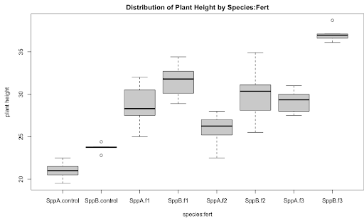
As a preliminary step in Exploratory Data Analysis (EDA), a side-by-side boxplot display of height vs. species organized by fertilizer type would be an ideal graphic. The plot below illustrates, the height differences between species are variable among fertilizer types; see for example the difference in height between SppA and SppB for Control is much less than that for F3. This indicates that fert*species could be a significant interaction prompting a factorial model with interaction.
To run the two-factor factorial model with interaction in SAS proc mixed, we can use:
/*Runs the two-factor factorial model with interaction*/
                proc mixed data=greenhouse_2way method=type3;
                class fert species;
                model height = fert species fert*species;
                store out2way;
                run;
Similar to when running the single factor ANOVA, the name of the dataset is specified in the proc mixed statement as well as the method=type3 option that specifies the way the F-test is calculated. The categorical factors fert and species are included in the class statement. The terms (or effects) in the model statement are consistent with the source effects in the layout of the "theoretical" ANOVA table illustrated in 5.1. Finally, the store command stores the elements necessary for the generation of the LS-means interval plot.
Recall the two ANOVA rules, applicable to any model: (1) the df values add up to total df and (2) the sums of squares add up to total sums of squares. As seen by the output below, the df values and sums of squares follow these rules. (It is easy to confirm that the total sum of squares = 1168.7325, by the 2nd ANOVA rule.)
Type 3 Analysis of Variance | ||||||||
|---|---|---|---|---|---|---|---|---|
Source | DF | Sum of Squares | Mean Square | Expected Mean Square | Error Term | Error DF | F Value | Pr > F |
fert | 3 | 745.437500 | 248.479167 | Var(Residual)+Q(fert,fert*species) | MS(Residual) | 40 | 73.10 | <.0001 |
species | 1 | 236.740833 | 236.740833 | Var(Residual)+Q(species,fert*species) | MS(Residual) | 40 | 69.65 | <.0001 |
fert*species | 3 | 50.584167 | 16.861389 | Var(Residual)+Q(fert*species) | MS(Residual) | 40 | 4.96 | 0.0051 |
Residual | 40 | 135.970000 | 3.399250 | Var(Residual) | ||||
*** RULE ***
In a model with the interaction effect, the interaction term should be interpreted first. If the interaction effect is significant, then do NOT interpret the main effects individually. Instead, compare the mean response differences among the different factor level combinations.
In general, a significant interaction effect indicates that the impact of the levels of Factor A on the response depends upon the level of Factor B and vice versa. In other words, in the presence of a significant interaction, a stand-alone main effect is of no consequence. In the case where an interaction is not significant, the interaction term can be dropped and a model without the interaction should be run. This model without the interaction is called the Additive Model and is discussed in the next section.
Applying the above rule for this example, the small p-value of 0.0051 displayed in the table above indicates that the interaction effect is significant suggesting the main effects of either fert and species should not be considered individually. It is the average response differences among the fert and species combinations that matter. In order to determine the statistically significant treatment combinations a suitable multiple comparison procedure (such as the Tukey procedure) can be performed on the LS-means of the interaction effect.
The necessary follow-up SAS code to perform this procedure is given below.
ods graphics on;
                proc plm restore=out2way;
                lsmeans fert*species / adjust=tukey plot=(diffplot(center)
                meanplot(cl ascending)) cl lines;
                /* Because the 2-factor interaction is significant, we work with
                the means for treatment combination*/
                run;
SAS Output for the LS-means:
fert*species Least Squares Means | |||||||||
|---|---|---|---|---|---|---|---|---|---|
fert | species | Estimate | Standard Error | DF | t Value | Pr > |t| | Alpha | Lower | Upper |
control | SppA | 21.0000 | 0.7527 | 40 | 27.90 | <.0001 | 0.05 | 19.4788 | 22.5212 |
control | SppB | 23.7000 | 0.7527 | 40 | 31.49 | <.0001 | 0.05 | 22.1788 | 25.2212 |
f1 | SppA | 28.6000 | 0.7527 | 40 | 38.00 | <.0001 | 0.05 | 27.0788 | 30.1212 |
f1 | SppB | 31.6167 | 0.7527 | 40 | 42.00 | <.0001 | 0.05 | 30.0954 | 33.1379 |
f2 | SppA | 25.8667 | 0.7527 | 40 | 34.37 | <.0001 | 0.05 | 24.3454 | 27.3879 |
f2 | SppB | 30.0500 | 0.7527 | 40 | 39.92 | <.0001 | 0.05 | 28.5288 | 31.5712 |
f3 | SppA | 29.2000 | 0.7527 | 40 | 38.79 | <.0001 | 0.05 | 27.6788 | 30.7212 |
f3 | SppB | 37.0667 | 0.7527 | 40 | 49.25 | <.0001 | 0.05 | 35.5454 | 38.5879 |
Note that the p-values here (Pr > t) are testing the hypotheses that the fert and species combination means = 0. This may be of very little interest. However, a comparison of mean response values for different species and fertilizer combinations may be more beneficial and can be derived from the diffogram shown in Figure 5.2. Again recall that if the confidence interval does not contain zero, then the difference between the two associated means is statistically significant.
Notice also that we see a single value for the standard error based on the MSE from the ANOVA rather than a separate standard error for each mean as we would get from proc summary for the sample means. In this example, with equal sample sizes and no covariates, the LS-means will be identical to the ordinary means displayed in the summary procedure.
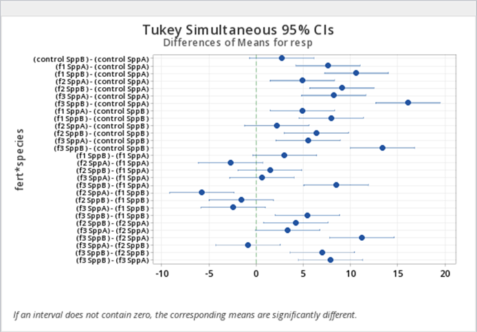
There are a total of 8 fert*species combinations resulting in a total of \({8 \choose 2} = 28\) pairwise comparisons. From the diffogram for differences in fert*species combinations, we see that 10 of them are not significant and 18 of them are significant at a 5% level after Tukey adjustment (more about diffograms). The information used to generate the diffogram is presented in the table for differences of fert*species least squares means in the SAS output (this table is not displayed here).
We can save the differences estimated in SAS proc mixed and utilize proc sgplot to create the plot of differences in mean response for the fert*species combinations as shown in Figure 5.3 (SAS code not provided in these notes). The CIs shown are the Tukey adjusted CIs and the interpretations are similar to what we observed from the diffogram in Figure 5.2.
In addition to comparing differences in mean responses for the fert*species combinations, the SAS code above will also produce the line plot for multiple comparisons of means for fert*species combinations (Figure 5.4) and the plot of means responses organized in the ascending order with 95% CIs for fert*species combinations (Figure 5.5).
The line plot Figure 5.4 connects groups in which the LS-means are not statistically different and displays a summary of which groups have similar means. The plot of means with 95% CIs in Figure 5.5 illustrates the same result, although it uses unadjusted CIs. The organization of the estimated mean responses in ascending order facilitates interpretation of the results.
Using LS-means subsequent to performing an ANOVA will help to identify the significantly different treatment level combinations. In other words, the analysis of a factorial model does not end with a p-value for an F-test. Rather, a small p-value signals the need for a mean comparison procedure.
For Minitab, we also need to convert the data to a stacked format (Lesson4 2 way Stacked Dataset). Once we do this, we will need to use a different set of commands to generate the ANOVA. We use...
Stat > ANOVA > General Linear Model > Fit General Linear Model
and get the following dialog box:
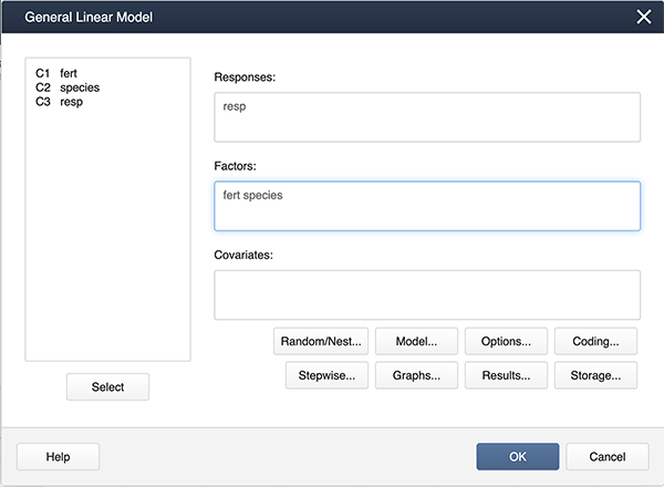
Click on Model…, hold down the shift key and highlight both factors. Then click on the Add box to add the interaction to the model.
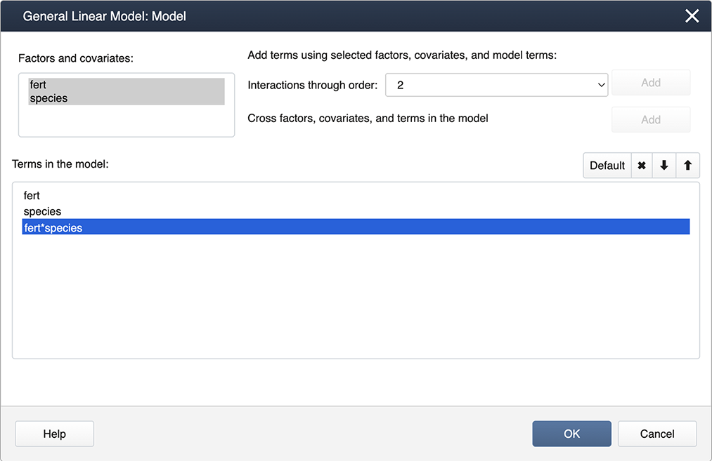
These commands will produce the ANOVA results below which are similar to the output generated by SAS (shown in the previous section).
Analysis of Variance
Source | DF | Adj SS | Adj MS | F-value | P-value |
|---|---|---|---|---|---|
fert | 3 | 745.44 | 248.479 | 73.10 | 0.000 |
species | 1 | 236.74 | 236.741 | 69.65 | 0.000 |
fert*species | 3 | 50.58 | 16.861 | 4.96 | 0.005 |
Error | 40 | 135.97 | 3.399 | ||
Total | 47 | 1168.73 |
Following the ANOVA run, you can generate the mean comparisons by
Stat > ANOVA > General Linear Model > Comparisons
Then specify the fert*species interaction term for the comparisons by checking the box.
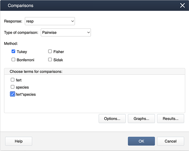
Then choose Graphs to get the following dialog box, where ‘Interval plot for difference of means’ should be checked.
The outputs are shown below.
Grouping Information Using the Tukey Method and 95% Confidence
fert | species | N | Mean | Grouping |
|---|---|---|---|---|
f3 | SppB | 6 | 37.0667 | A |
f1 | SppB | 6 | 31.6167 | B |
f2 | SppB | 6 | 30.0500 | B |
f3 | SppA | 6 | 29.2000 | B C |
f1 | SppA | 6 | 28.6000 | B C |
f2 | SppA | 6 | 25.8667 | C D |
control | SppB | 6 | 23.7000 | D E |
control | SppA | 6 | 21.0000 | E |
Means that do not share a letter are significantly different.
First, load and attach the greenhouse data in R.
setwd("~/path-to-folder/")
                        greenhouse_2way_data <-read.table("greenhouse_2way_data.txt",header=T)
                        attach(greenhouse_2way_data)
We can then produce a boxplot of species organized by fertilizer.
boxplot(resp~species:fert, main = "Distribution of Plant Height by Species:Fert",
                                xlab = "species:fert", ylab = "plant height")
Next, we fit the two-way interaction model and obtain the ANOVA table.
options(contrasts=c("contr.sum","contr.poly"))
                        lm1 = lm(resp ~ species + fert + fert:species) # equivalent to lm1 = lm(resp ~ fert*species)
                        aov3 = car::Anova(lm1, type=3) # equivalent to library(car); aov3 = Anova(lm1, type=3)
                        print(aov3, digits=7)
Anova Table (Type III tests)
Response: resp
Sum Sq Df F value Pr(>F)
(Intercept) 38680.81 1 11379.21821 < 2.22e-16 ***
species 236.74 1 69.64502 2.7065e-10 ***
fert 745.44 3 73.09823 2.7657e-16 ***
species:fert 50.58 3 4.96033 0.0050806 **
Residuals 135.97 40
---
Signif. codes: 0 ‘***’ 0.001 ‘**’ 0.01 ‘*’ 0.05 ‘.’ 0.1 ‘ ’ 1 We can examine the LS means interval plot of the interaction as follows:
 aov1 = aov(lm1)
                        lsmeans = emmeans::emmeans(aov1, ~fert:species)
                        lsmeans
                        plot(lsmeans, xlab="height LS-Means with 95% CIs")
fert species emmean SE df lower.CL upper.CL
control SppA 21.0 0.753 40 19.5 22.5
f1 SppA 28.6 0.753 40 27.1 30.1
f2 SppA 25.9 0.753 40 24.3 27.4
f3 SppA 29.2 0.753 40 27.7 30.7
control SppB 23.7 0.753 40 22.2 25.2
f1 SppB 31.6 0.753 40 30.1 33.1
f2 SppB 30.1 0.753 40 28.5 31.6
f3 SppB 37.1 0.753 40 35.5 38.6
Confidence level used: 0.95 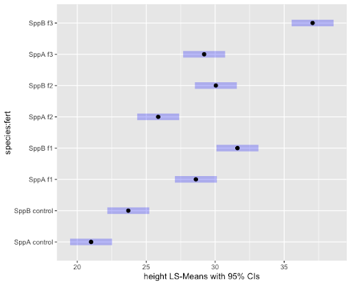
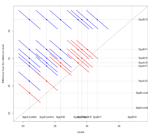
The Tukey pairwise comparisons of means with 95% family-wise confidence can be examined with the following commands. Note we use the bounds of the CIs (computed by the TukeyHSD function) to create a color coding based on significance.
tpairs = TukeyHSD(aov1)
                        col1 = rep("blue",nrow(tpairs$`species:fert`))
                        col1[tpairs$`species:fert`[,2]<0 & tpairs$`species:fert`[,3]>0] = "red"
                        plot(tpairs,col=col1)
There are several packages that can be used to obtain the Tukey groups and diffogram. An example using the sasLM package is as follows.
library(sasLM)LSM(lm1, Data = greenhouse_2way_data, Term = "species:fert", adj = "tukey")
                        Diffogram(lm1, Data = greenhouse_2way_data, Term = "species:fert", adj = "tukey")
Group LSmean LowerCL UpperCL SE Df
SppB:f3 A 37.06667 35.54542 38.58791 0.7526896 40
SppB:f1 B 31.61667 30.09542 33.13791 0.7526896 40
SppB:f2 B 30.05000 28.52876 31.57124 0.7526896 40
SppA:f3 BC 29.20000 27.67876 30.72124 0.7526896 40
SppA:f1 BC 28.60000 27.07876 30.12124 0.7526896 40
SppA:f2 CD 25.86667 24.34542 27.38791 0.7526896 40
SppB:control DE 23.70000 22.17876 25.22124 0.7526896 40
SppA:control E 21.00000 19.47876 22.52124 0.7526896 40