How does Minitab handle these types of experiments? Section
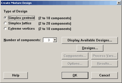
Mixture designs are a special case of response surface designs. Under the stat menu in many tab, select design of experiments, then mixture, create mixture design. Minitab then presents you with the following dialog box:

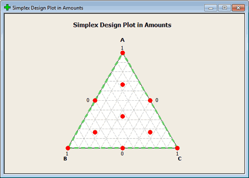
Simplex lattice option will look at the points that are extremes. Simplex lattice creates a design for p components of degree m. In this case, we want points that are made up of 0, \(1/m, 2/m, \dots\) up to 1. Classifying the points in this way tells us how we will space the points. For instance, if m = 2, then the only points we would have would be 0, 1/2, and 1 to play with in all key dimensions. You can create this design in Minitab, for 3 factors, using tab Stat > DOE > Mixture > Create Mixture Design and select Simplex Centroid. See the image here:

If we are in a design with the m = 3, then we would have 0, 1/3, 2/3, and 1. In this case we would have points a third of the way along each dimension. Any point on the boundary can be constructed in this way.
All of these points are on the boundary which means that they are made up of mixtures that omit one of the components. (This is not always desirable but in some settings it is fine.)
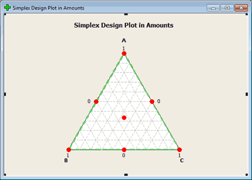
The centroid is the point in the middle. Axial points are points that lie along the lines that intersect the region of experimentation, points that are located interior and therefore include part of all of the components.
You can create this design in Minitab, for 3 factors, using tab Stat > DOE > Mixture > Create Mixture Design and select Simplex Centroid. See the image here:

This should give you the range of points that you think of when designing in a mixture. again, you want points in the middle but like regression in an unconstrained space you typically want to have your points farther out so you have good leverage. From this perspective, the points on the outside make a lot of sense. From an actual experimentation situation, you would have to be in a scientific setting also where those points make sense. If not, we would constrain this region to begin with. We will get in to this later.
How Rich of a Design? Section
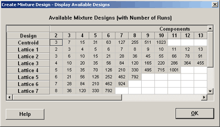
Let's look at the set of possible designs that Minitab gives us.

Where it is labeled on the left Lattice 1, Lattice 2, etc., here minitab is referring to degree 1, 2, etc. So, if you want a lattice of degree 1, this is not very interesting. This means that you just have a 0 and 1. If you go to a lattice of degree 2 then you need six points in three dimensions. This is pretty much what we looked at previously... (roll over the red mixture points, below).
| Run | Type | A | B | C |
|---|---|---|---|---|
| 1 | 1 | 1.0000 | 0.0000 | 0.0000 |
| 2 | 2 | 0.5000 | 0.5000 | 0.0000 |
| 3 | 2 | 0.5000 | 0.0000 | 0.5000 |
| 4 | 1 | 0.0000 | 1.0000 | 0.0000 |
| 5 | 2 | 0.0000 | 0.5000 | 0.5000 |
| 6 | 1 | 0.0000 | 0.0000 | 1.0000 |
Here is a design table for a lattice with degree 3:
| Run | Type | A | B | C |
|---|---|---|---|---|
| 1 | 1 | 1.0000 | 0.0000 | 0.0000 |
| 2 | 2 | 0.6667 | 0.3333 | 0.0000 |
| 3 | 2 | 0.6667 | 0.0000 | 0.3333 |
| 4 | 2 | 0.3333 | 0.6667 | 0.0000 |
| 5 | 0 | 0.3333 | 0.3333 | 0.3333 |
| 6 | 2 | 0.3333 | 0.0000 | 0.6667 |
| 7 | 1 | 0.0000 | 1.0000 | 0.0000 |
| 8 | 2 | 0.0000 | 0.6667 | 0.3333 |
| 9 | 2 | 0.0000 | 0.3333 | 0.6667 |
| 10 | 1 | 0.0000 | 0.0000 | 1.0000 |
Now let's go into Minitab and augment this design by including axial points. Here is what results:
| Run | Type | A | B | C |
|---|---|---|---|---|
| 1 | 1 | 1.0000 | 0.0000 | 0.0000 |
| 2 | 2 | 0.6667 | 0.3333 | 0.0000 |
| 3 | 2 | 0.6667 | 0.0000 | 0.3333 |
| 4 | 2 | 0.3333 | 0.6667 | 0.0000 |
| 5 | 0 | 0.3333 | 0.3333 | 0.3333 |
| 6 | 2 | 0.3333 | 0.0000 | 0.6667 |
| 7 | 1 | 0.0000 | 1.0000 | 0.0000 |
| 8 | 2 | 0.0000 | 0.6667 | 0.3333 |
| 9 | 2 | 0.0000 | 0.3333 | 0.6667 |
| 10 | 1 | 0.0000 | 0.0000 | 1.0000 |
| 11 | -1 | 0.6667 | 0.1667 | 0.6667 |
| 12 | -1 | 0.1667 | 0.6667 | 0.1667 |
| 13 | -1 | 0.1667 | 0.1667 | 0.6667 |
This gives us three more points. Each of these points is 2/3, 1/6, 1/6. These are interior points.
These are good designs if you can run your experiment in the whole region.
Let's take a look at four dimensions and see what the program will do here. Here is a design with four components, four dimensions, and a lattice of degree three. We have also selected to augment this design with axial and center points.
| Run | Type | A | B | C | D |
|---|---|---|---|---|---|
| 1 | 1 | 1.0000 | 0.0000 | 0.0000 | 0.0000 |
| 2 | 2 | 0.6667 | 0.3333 | 0.0000 | 0.0000 |
| 3 | 2 | 0.6667 | 0.0000 | 0.3333 | 0.0000 |
| 4 | 2 | 0.6667 | 0.0000 | 0.0000 | 0.3333 |
| 5 | 2 | 0.3333 | 0.6667 | 0.0000 | 0.0000 |
| 6 | 3 | 0.3333 | 0.3333 | 0.3333 | 0.0000 |
| 7 | 3 | 0.3333 | 0.3333 | 0.0000 | 0.3333 |
| 8 | 2 | 0.3333 | 0.0000 | 0.6667 | 0.0000 |
| 9 | 3 | 0.3333 | 0.0000 | 0.3333 | 0.3333 |
| 10 | 2 | 0.3333 | 0.0000 | 0.0000 | 0.6667 |
| 11 | 1 | 0.0000 | 1.0000 | 0.0000 | 0.0000 |
| 12 | 2 | 0.0000 | 0.6667 | 0.3333 | 0.0000 |
| 13 | 2 | 0.0000 | 0.6667 | 0.0000 | 0.3333 |
| 14 | 2 | 0.0000 | 0.3333 | 0.6667 | 0.0000 |
| 15 | 3 | 0.0000 | 0.3333 | 0.3333 | 0.3333 |
| 16 | 2 | 0.0000 | 0.3333 | 0.0000 | 0.6667 |
| 17 | 1 | 0.0000 | 0.0000 | 1.0000 | 0.0000 |
| 18 | 2 | 0.0000 | 0.0000 | 0.6667 | 0.3333 |
| 19 | 2 | 0.0000 | 0.0000 | 0.3333 | 0.6667 |
| 20 | 1 | 0.0000 | 0.0000 | 0.0000 | 1.0000 |
| 21 | 0 | 0.2500 | 0.2500 | 0.2500 | 0.2500 |
| 22 | -1 | 0.6250 | 0.1250 | 0.1250 | 0.1250 |
| 23 | -1 | 0.1250 | 0.6250 | 0.1250 | 0.1250 |
| 24 | -1 | 0.1250 | 0.1250 | 0.6250 | 0.1250 |
| 25 | -1 | 0.1250 | 0.1250 | 0.1250 | 0.6250 |
This gives us 25 points in the design and the plot shows us the four faces of the tetrahedron. It doesn't look like it is showing us a plot of the interior points.