In the previous section, we saw a \(2^2\) treatment design with 4 runs constructed in two blocks confounded with the AB contrast. We also saw a \(2^3\) design constructed in two blocks, with ABC confounded with blocks. We say this is a \(2^3\) design in \(2^1\) blocks of size \(2^2\) per replicate. And we also saw a \(2^3\) design in \(2^2 = 4\) blocks of size \(2^1 = 2\) per replicate with effects AB, AC, and therefore \(AB \times AC = A^{2}BC = BC\) confounded with blocks.
Now let’s consider this last situation when we have \(n = 3\) replicates of this basic design with \(b = 4\) blocks. We can write a model:
\(Y_{ijklm}= \mu+r_{i}+b_{j(i)}+\alpha_{k}+\beta_{l}+\gamma_{m}+...\)
where “i” is the index for replicates and “j” is the index for blocks within the replicates. “k”, “l” and “m” are indices for the different treatment factors.
| AOV | df | |
|---|---|---|
| Rep | n-1 | = 3 - 1 = 2 |
| Blk(Rep) | n(b - 1) | = 3(4 - 1) = 9 |
| A | 2 - 1 | 1 |
| B | 2 - 1 | 1 |
| C | 2 - 1 | 1 |
| ABC | 2 - 1 | 1 |
| Error | (n - 1)*4 | 8 |
| Total | \(n*2^{3} - 1\) | 23 |
Now we consider another example: in figure 7.3 of the text we see four replicates with ABC confounded in each of the four replicates. The ANOVA for this design is seen in table 7.5 which shows that the Block effect (Block 1 vs. Block 2) is equivalent to the ABC effect and since there are four replicates of this basic design, we can extract some information about the ABC effect, and indeed test the hypothesis of no ABC effect, by using the Rep × ABC interaction as error.
See the analysis of this design using Minitab:
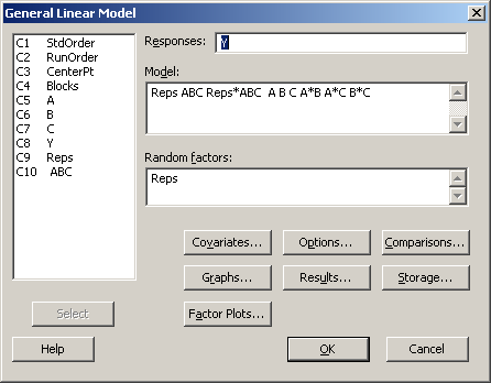
Stat > ANOVA > General Linear Model
and fitting the following model:

If Reps is specified as a random effects factor in the model, as above, GLM will produce the correct F-tests based on the Expected Means Squares. The reason is analogous to the RCBD with random blocks (Reps) and a fixed treatment (ABC). The topic of random factors is completely covered in chapter 13 of the text book
For Minitab Stat > ANOVA > GLM to analyze this data, you need to first construct a pseudo-factor called "ABC" which is constructed by multiplying the levels of A, B, and C using 'Calculator' under the 'Data' menu in Minitab. Click on the 'Inspect' button below which will walk you through this process using Minitab v.16.
In addition you can open this Minitab project file 2-k-confound-ABC.mpx and review the steps leading to the output. The response variable Y is random data simply to illustrate the analysis.
Here is an alternative way to analyze this design using the analysis portion of the fractional factorial software in Minitab v.16.
A similar exercise can be done to illustrate the confounded situation where the main effect, say A, is confounded with blocks. Again, since this is a bit nonstandard, we will need to generate a design in Minitab using the default settings and then edit the worksheet to create the confounding we desire and analyze it in GLM.