Minitab®
Consider the cloth dyes data from Problem 5.19 in the text:
For each combination of time, temperature and operator, there are three observations. Now we have a case where there are three factors and three observations per cell. Let's run this model in Minitab.
General Linear Model: Score versus Temperature, Cycle Time, Operator
| Factor | Type | Levels | Values |
|---|---|---|---|
| Temperature | fixed | 2 | 300, 350 |
| Cycle Time | fixed | 3 | 40, 50, 60 |
| Operator | fixed | 3 | 1, 2, 3 |
Analysis of Variance for Score, using Adjusted SS for Tests
| Source | DF | Seq SS | Adj SS | Adj MS | F | P |
|---|---|---|---|---|---|---|
| Temperature | 1 | 50.074 | 50.074 | 50.074 | 15.28 | 0.000 |
| Cycle Time | 2 | 436.000 | 436.000 | 218.000 | 66.51 | 0.000 |
| Operator | 2 | 261.333 | 261.333 | 130.667 | 39.86 | 0.000 |
| Temperature*Cycle Time | 2 | 78.815 | 78.815 | 39.407 | 12.02 | 0.000 |
| Temperature*Operator | 2 | 11.259 | 11.259 | 5.630 | 1.72 | 0.194 |
| Cycle Time*Operator | 4 | 355.667 | 355.667 | 88.917 | 27.13 | 0.000 |
| Temperature*Cycle Time*Operator | 4 | 46.185 | 46.185 | 11.546 | 3.52 | 0.016 |
| Error | 36 | 118.000 | 118.000 | 3.278 | ||
| Total | 53 | 1357.333 | ||||
| S = 1.81046 R-Sq = 91.31% R-Sq(adj) = 87.20% | ||||||
Unusual Observations for Score
| Obs | Score | Fit | SE Fit | Residual | St Resid |
|---|---|---|---|---|---|
| 5 | 34.0000 | 37.0000 | 1.0453 | -3.0000 | -2.03 R |
| 46 | 28.0000 | 25.0000 | 1.0453 | 3.0000 | 2.03 R |
| R denotes an observation with a large standardized residual. | |||||
The ANOVA table shows us that the main effects due to cycle time, operator, and temperature are all significant. The two-way interactions for cycle time by operator and cycle time by temperature are significant. But the operator by temperature is not significant but the dreaded three-way interaction is significant. What does it mean when a three-way interaction is significant?
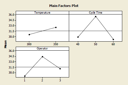
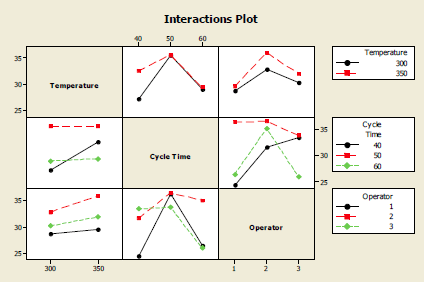
Let's take a look at the factor plots:


These interaction plots show us the three sets of two-way cell means, each of the three are plotted in two different ways. This is a useful plot to try to understand what is going on. These are all the two-way plots.
Typically a three-way interaction would be plotted as two panels... showing how the two-way interactions differ across the levels of the third factor. Minitab does not do that for you automatically.
Let's think about how this experiment was done. There are three observations for each combination of factors. Are they actually separate experimental units or are they simply three measurements on the same experimental unit? If they are simply three measurements on the same piece of cloth that was all done in the same batch, for instance, then they are not really independent. If this is the case, then another way to look at this data would be to average those replications. In this case there is only 1 observation for each treatment, so that there would be no d.f. for error. However, the way the problem is presented in the text, they appear to have been treated independently and thus are true replicates, leading to 36 d.f. for error.
You could also think about the operator not as a factor that you're interested in but more as a block factor, i.e. a source of variation that we want to remove from the study. What we're really interested in is the effect of temperature and time on the process of dyeing the cloth. In this case we could think about using the operator as a block effect. Running the analysis again, now we get the same plot but look at the ANOVA table: now the interactions related to operator have been pooled as a part of the error. So the residual error term now has 2 + 4 + 4 + 36 = 46 df for error. Note also that if you do use the operator as a treatment factor, it probably should be considered random. In this case, you would probably want to consider the 2 and 3-way interactions involving operator to be random effects. Experiments in which some factors are fixed and others are random are called mixed effects experiments. The analysis of mixed effects experiments is discussed in Chapter 13.
General Linear Model: Score versus Temperature, Cycle Time, Operator
| Factor | Type | Levels | Values |
|---|---|---|---|
| Temperature | fixed | 2 | 300, 350 |
| Cycle Time | fixed | 3 | 40, 50, 60 |
| Operator | fixed | 3 | 1, 2, 3 |
Analysis of Variance for Score, using Adjusted SS for Tests
| Source | DF | Seq SS | Adj SS | Adj MS | F | P |
|---|---|---|---|---|---|---|
| Temperature | 1 | 50.07 | 50.07 | 50.07 | 4.34 | 0.043 |
| Cycle Time | 2 | 436.00 | 436.00 | 218.00 | 18.88 | 0.000 |
| Operator | 2 | 261.33 | 261.33 | 130.67 | 11.32 | 0.000 |
| Temperature*Cycle Time | 2 | 78.81 | 78.81 | 39.41 | 11.32 | 0.041 |
| Error | 46 | 531.11 | 531.11 | 11.55 | ||
| Total | 53 | 1357.33 | ||||
| S = 3.39792 R-Sq = 60.87% R-Sq(adj) = 54.92% | ||||||
Unusual Observations for Score
| Obs | Score | Fit | SE Fit | Residual | St Resid |
|---|---|---|---|---|---|
| 28 | 23.0000 | 30.1111 | 1.3079 | -7.1111 | -2.27 R |
| 48 | 39.0000 | 32.1111 | 1.3079 | 6.8889 | 2.20 R |
| R denotes an observation with a large standardized residual. | |||||
What this points out is the importance of distinguishing what is a block factor, and which are the treatment factors when you have a multifactor experimental design. This should be apparent from how the experiment was conducted, but if the data are already collected when you are introduced to the problem, you need to inquire carefully to understand how the experiment was actually conducted to know what model to use in the analysis.
Let's take a look two examples using this same dataset using Minitab v19. First we will analyze the quantitative factors involved, Cycle Time and Temperature and as though they were qualitative - simply nominal factors.
Next, using Operator as a block we will now use Minitab v19 to treat the quantitative factors as qualitative factors and apply these in a regression analysis.