To compare the results from the RCBD, we take a look at the table below. What we did here was use the one-way analysis of variance instead of the two-way to illustrate what might have occurred if we had not blocked, if we had ignored the variation due to the different specimens. Blocking is a technique for dealing with nuisance factors.
A nuisance factor is a factor that has some effect on the response, but is of no interest to the experimenter; however, the variability it transmits to the response needs to be minimized or explained. We will talk about treatment factors, which we are interested in, and blocking factors, which we are not interested in. We will try to account for these nuisance factors in our model and analysis.
Typical nuisance factors include batches of raw material if you are in a production situation, different operators, nurses or subjects in studies, the pieces of test equipment, when studying a process, and time (shifts, days, etc.) where the time of the day or the shift can be a factor that influences the response.
Many industrial and human subjects experiments involve blocking, or when they do not, probably should in order to reduce the unexplained variation.
Where does the term block come from? The original use of the term block for removing a source of variation comes from agriculture. Given that you have a plot of land and you want to do an experiment on crops, for instance perhaps testing different varieties or different levels of fertilizer, you would take a section of land and divide it into plots and assigned your treatments at random to these plots. If the section of land contains a large number of plots, they will tend to be very variable - heterogeneous.
A block is characterized by a set of homogeneous plots or a set of similar experimental units. In agriculture a typical block is a set of contiguous plots of land under the assumption that fertility, moisture, weather, will all be similar, and thus the plots are homogeneous.
Failure to block is a common flaw in designing an experiment. Can you think of the consequences?
If the nuisance variable is known and controllable, we use blocking and control it by including a blocking factor in our experiment.
If you have a nuisance factor that is known but uncontrollable, sometimes we can use analysis of covariance (see Chapter 15) to measure and remove the effect of the nuisance factor from the analysis. In that case we adjust statistically to account for a covariate, whereas in blocking, we design the experiment with a block factor as an essential component of the design. Which do you think is preferable?
Many times there are nuisance factors that are unknown and uncontrollable (sometimes called a “lurking” variable). We use randomization to balance out their impact. We always randomize so that every experimental unit has an equal chance of being assigned to a given treatment. Randomization is our insurance against a systematic bias due to a nuisance factor.
Sometimes several sources of variation are combined to define the block, so the block becomes an aggregate variable. Consider a scenario where we want to test various subjects with different treatments.
Age classes and gender
In studies involving human subjects, we often use gender and age classes as the blocking factors. We could simply divide our subjects into age classes, however this does not consider gender. Therefore we partition our subjects by gender and from there into age classes. Thus we have a block of subjects that is defined by the combination of factors, gender and age class.
Institution (size, location, type, etc)
Often in medical studies, the blocking factor used is the type of institution. This provides a very useful blocking factor, hopefully removing institutionally related factors such as size of the institution, types of populations served, hospitals versus clinics, etc., that would influence the overall results of the experiment.
Example 4.1: Hardness Testing Section
In this example we wish to determine whether 4 different tips (the treatment factor) produce different (mean) hardness readings on a Rockwell hardness tester. The treatment factor is the design of the tip for the machine that determines the hardness of metal. The tip is one component of the testing machine.
To conduct this experiment we assign the tips to an experimental unit; that is, to a test specimen (called a coupon), which is a piece of metal on which the tip is tested.
If the structure were a completely randomized experiment (CRD) that we discussed in lesson 3, we would assign the tips to a random piece of metal for each test. In this case, the test specimens would be considered a source of nuisance variability. If we conduct this as a blocked experiment, we would assign all four tips to the same test specimen, randomly assigned to be tested on a different location on the specimen. Since each treatment occurs once in each block, the number of test specimens is the number of replicates.
Back to the hardness testing example, the experimenter may very well want to test the tips across specimens of various hardness levels. This shows the importance of blocking. To conduct this experiment as a RCBD, we assign all 4 tips to each specimen.
In this experiment, each specimen is called a “block”; thus, we have designed a more homogenous set of experimental units on which to test the tips.
Variability between blocks can be large, since we will remove this source of variability, whereas variability within a block should be relatively small. In general, a block is a specific level of the nuisance factor.
Another way to think about this is that a complete replicate of the basic experiment is conducted in each block. In this case, a block represents an experimental-wide restriction on randomization. However, experimental runs within a block are randomized.
Suppose that we use b = 4 blocks as shown in the table below:
| Test Coupon (Block) | |||
|---|---|---|---|
| 1 | 2 | 3 | 4 |
| Tip 3 | Tip 3 | Tip 2 | Tip 1 |
| Tip 1 | Tip 4 | Tip 1 | Tip 4 |
| Tip 4 | Tip 2 | Tip 3 | Tip 3 |
| Tip 2 | Tip 1 | Tip 4 | Tip 3 |
Notice the two-way structure of the experiment. Here we have four blocks and within each of these blocks is a random assignment of the tips within each block.
We are primarily interested in testing the equality of treatment means, but now we have the ability to remove the variability associated with the nuisance factor (the blocks) through the grouping of the experimental units prior to having assigned the treatments.
The ANOVA for Randomized Complete Block Design (RCBD) Section
In the RCBD we have one run of each treatment in each block. In some disciplines, each block is called an experiment (because a copy of the entire experiment is in the block) but in statistics, we call the block to be a replicate. This is a matter of scientific jargon, the design and analysis of the study is an RCBD in both cases.
Suppose that there are a treatments (factor levels) and b blocks.
A statistical model (effects model) for the RCBD is:
\(Y_{ij}=\mu +\tau_i+\beta_j+\varepsilon_{ij}
\left\{\begin{array}{c}
i=1,2,\ldots,a \\
j=1,2,\ldots,b
\end{array}\right. \)
This is just an extension of the model we had in the one-way case. We have for each observation \(Y_{ij}\) an additive model with an overall mean, plus an effect due to treatment, plus an effect due to block, plus error.
The relevant (fixed effects) hypothesis for the treatment effect is:
\(H_0:\mu_1=\mu_2=\cdots=\mu_a \quad \mbox{where}
\quad \mu_i=(1/b)\sum\limits_{j=1}^b (\mu+\tau_i+\beta_j)=\mu+\tau_i\)
\(\mbox{if}\quad \sum\limits_{j=1}^b \beta_j =0\)
We make the assumption that the errors are independent and normally distributed with constant variance \(\sigma^2\).
The ANOVA is just a partitioning of the variation:
\begin{eqnarray*} \sum\limits_{i=1}^a \sum\limits_{j=1}^b (y_{ij}-\bar{y}_{..})^2 &=& \sum\limits_{i=1}^a \sum\limits_{j=1}^b [(\bar{y}_{i.}-\bar{y}_{..})+(\bar{y}_{.j}-\bar{y}_{..}) \\ & & +(y_{ij}-\bar{y}_{i.}-\bar{y}_{.j}+\bar{y}_{..})]^2\\ &=& b\sum\limits_{i=1}{a}(\bar{y}_{i.}-\bar{y}_{..})^2+a\sum\limits_{j=1}{b}(\bar{y}_{.j}-\bar{y}_{..})^2\\ & & +\sum\limits_{i=1}^a \sum\limits_{j=1}^b (y_{ij}-\bar{y}_{i.}-\bar{y}_{.j}+\bar{y}_{..})^2 \end{eqnarray*}
\(SS_T=SS_{Treatments}+SS_{Blocks}+SS_E\)
The algebra of the sum of squares falls out in this way. We can partition the effects into three parts: sum of squares due to treatments, sum of squares due to the blocks and the sum of squares due to error.
The degrees of freedom for the sums of squares in:
\(SS_T=SS_{Treatments}+SS_{Blocks}+SS_E\)
are as follows for a treatments and b blocks:
\(ab-1=(a-1)+(b-1)+(a-1)(b-1)\)
The partitioning of the variation of the sum of squares and the corresponding partitioning of the degrees of freedom provides the basis for our orthogonal analysis of variance.
ANOVA Display for the RCBD
| Source of Variation |
Sum of Squares | Degrees of Freedom |
Mean Square | \(F_{0}\) |
|---|---|---|---|---|
| Treatments | \(SS_{Treatments}\) | \(a-1\) | \(\dfrac{SS_{Treatments}}{a-1}\) | \(\dfrac{MS_{Treatments}}{MS_{g}}\) |
| Blocks | \(SS_{Blocks}\) | \(b-1\) | \(\dfrac{SS_{Blocks}}{b-1}\) | |
| Error | \(SS_{E}\) | \((a-1)(b-1)\) | \(\dfrac{SS_{g}}{(a-1)(b-1)}\) | |
| Total | \(SS_{T}\) | \(N-1\) | ||
| Table 4-2 Analysis of Variance for a Randomized Complete Block Design | ||||
In Table 4.2 we have the sum of squares due to treatment, the sum of squares due to blocks, and the sum of squares due to error. The degrees of freedom add up to a total of N-1, where N = ab. We obtain the Mean Square values by dividing the sum of squares by the degrees of freedom.
Then, under the null hypothesis of no treatment effect, the ratio of the mean square for treatments to the error mean square is an F statistic that is used to test the hypothesis of equal treatment means.
The text provides manual computing formulas; however, we will use Minitab to analyze the RCBD.
Back to the Tip Hardness example:
Remember, the hardness of specimens (coupons) is tested with 4 different tips.
Here is the data for this experiment (tip_hardness.csv):
| Obs | Tip | Hardness | Coupon |
|---|---|---|---|
| 1 | 1 | 9.3 | 1 |
| 2 | 1 | 9.4 | 2 |
| 3 | 1 | 9.6 | 3 |
| 4 | 1 | 10.0 | 4 |
| 5 | 2 | 9.4 | 1 |
| 6 | 2 | 9.3 | 2 |
| 7 | 2 | 9.8 | 3 |
| 8 | 2 | 9.9 | 4 |
| 9 | 3 | 9.2 | 1 |
| 10 | 3 | 9.4 | 2 |
| 11 | 3 | 9.5 | 3 |
| 12 | 3 | 9.7 | 4 |
| 13 | 4 | 9.7 | 1 |
| 14 | 4 | 9.6 | 2 |
| 15 | 4 | 10.0 | 3 |
| 16 | 4 | 10.2 | 4 |
Here is the output from Minitab. We can see four levels of the Tip and four levels for Coupon:
The Analysis of Variance table shows three degrees of freedom for Tip three for Coupon, and the error degrees of freedom is nine. The ratio of mean squares of treatment over error gives us an F ratio that is equal to 14.44 which is highly significant since it is greater than the .001 percentile of the F distribution with three and nine degrees of freedom.
| Factor | Type | Levels | Values |
|---|---|---|---|
| Tip | fixed | 4 | 1, 2, 3, 4 |
| Coupon | fixed | 4 | 1, 2, 3, 4 |
Analysis of Variance for Hardness
| Source | DF | SS | MS | F | P |
|---|---|---|---|---|---|
| Tip | 3 | 0.38500 | 0.12833 | 14.44 | 0.001 |
| Coupon | 3 | 0.82500 | 0.27500 | 30.94 | 0.000 |
| Error | 9 | 0.0800 | 0.00889 | ||
| Total | 15 | 1.29000 | |||
| S = 0.0942809 R-Sq = 93.80% R-Sq(adj) = 89.66% | |||||
Our 2-way analysis also provides a test for the block factor, Coupon. The ANOVA shows that this factor is also significant with an F-test = 30.94. So, there is a large amount of variation in hardness between the pieces of metal. This is why we used specimen (or coupon) as our blocking factor. We expected in advance that it would account for a large amount of variation. By including block in the model and in the analysis, we removed this large portion of the variation, such that the residual error is quite small. By including a block factor in the model, the error variance is reduced, and the test on treatments is more powerful.
The test on the block factor is typically not of interest except to confirm that you used a good blocking factor. The results are summarized by the table of means given below.
Means
| Tip | N | Hardness | Coupon | N | Hardness |
|---|---|---|---|---|---|
| 1 | 4 | 9.5750 | 1 | 4 | 9.4000 |
| 2 | 4 | 9.6000 | 3 | 4 | 9.4250 |
| 3 | 4 | 9.4500 | 3 | 4 | 9.7250 |
| 4 | 4 | 9.8750 | 4 | 4 | 9.9500 |
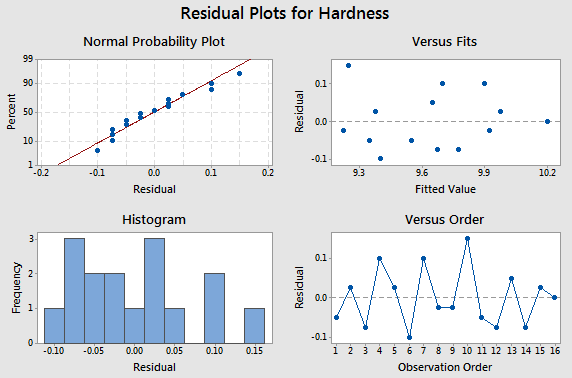
Here is the residual analysis from the two-way structure.
Comparing the CRD to the RCBD Section
To compare the results from the RCBD, we take a look at the table below. What we did here was use the one-way analysis of variance instead of the two-way to illustrate what might have occurred if we had not blocked, if we had ignored the variation due to the different specimens.
ANOVA: Hardness versus Tip
| Factor | Type | Levels | Values |
|---|---|---|---|
| Tip | fixed | 4 | 1, 2, 3, 4 |
Analysis of Variance for Hardness
| Source | DF | SS | MS | F | P |
|---|---|---|---|---|---|
| Tip | 3 | 0.38500 | 0.12833 | 1.70 | 0.220 |
| Error | 12 | 0.90500 | 0.07542 | ||
| Total | 15 | 1.29000 | |||
| S = 0.274621 R-Sq = 29.84% R-Sq(adj) = 12.31% | |||||
This isn't quite fair because we did in fact block, but putting the data into one-way analysis we see the same variation due to tip, which is 3.85. So we are explaining the same amount of variation due to the tip. That has not changed. But now we have 12 degrees of freedom for error because we have not blocked and the sum of squares for error is much larger than it was before, thus our F-test is 1.7. If we hadn't blocked the experiment our error would be much larger and in fact, we would not even show a significant difference among these tips. This provides a good illustration of the benefit of blocking to reduce error. Notice that the standard deviation, \(S=\sqrt{MSE}\), would be about three times larger if we had not blocked.
Other Aspects of the RCBD Section
The RCBD utilizes an additive model – one in which there is no interaction between treatments and blocks. The error term in a randomized complete block model reflects how the treatment effect varies from one block to another.
Both the treatments and blocks can be looked at as random effects rather than fixed effects, if the levels were selected at random from a population of possible treatments or blocks. We consider this case later, but it does not change the test for a treatment effect.
What are the consequences of not blocking if we should have? Generally the unexplained error in the model will be larger, and therefore the test of the treatment effect less powerful.
How to determine the sample size in the RCBD? The OC curve approach can be used to determine the number of blocks to run. The number of blocks, b, represents the number of replications. The power calculations that we looked at before would be the same, except that we use b rather than n, and we use the estimate of error, \(\sigma^{2}\), that reflects the improved precision based on having used blocks in our experiment. So, the major benefit or power comes not from the number of replications but from the error variance which is much smaller because you removed the effects due to block.