Simple comparative experiments are not only preliminary to this course but this takes you back probably into your first course in statistics. We will look at both hypothesis testing and estimation and from these perspectives, we will look at sample size determination.
Two Sample Experiment
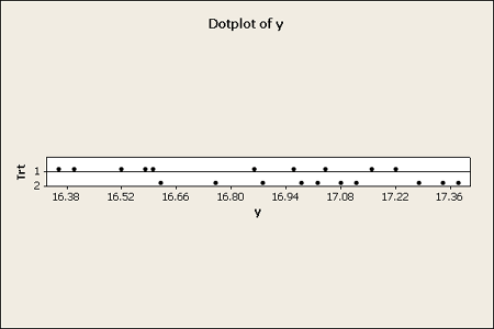
Here is an example from the text where there are two formulations for making cement mortar. It is hard to get a sense of the data when looking only at a table of numbers. You get a much better understanding of what it is about when looking at a graphical view of the data.

Dot plots work well to get a sense of the distribution. These work especially well for very small sets of data.
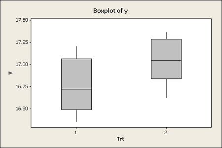
Another graphical tool is the boxplot, useful for small or larger data sets. If you look at the box plot you get a quick snapshot of the distribution of the data.

Remember that the box spans the middle 50% of the data (from the 25th to the 75th percentile) and the whiskers extend as far out as the minimum and maximum of the data, to a maximum of 1.5 times the width of the box, or 1.5 times the Interquartile range. So if the data are normal you would expect to see just the box and whisker with no dots outside. Potential outliers will be displayed as single dots beyond the whiskers.
This example is a case where the two groups are different in terms of the median, which is the horizontal line in the box. One cannot be sure simply by visualizing the data if there is a significant difference between the means of these two groups. However, both the box plots and the dot plot hint at differences.
Testing: The two sample t-test Section
For the two-sample t-test, both samples are assumed to come from Normal populations with (possibly different) means \(\mu_i\) and variances \(\sigma^2\). When the variances are not equal we will generally try to overcome this by transforming the data. Using a metric where the variation is equal we can use complex ANOVA models, which also assume equal variances. (There is a version of the two sample t-test which can handle different variances, but unfortunately, this does not extend to more complex ANOVA models.) We want to test the hypothesis that the means \(\mu_i\) are equal.
Our first look at the data above shows that the means are somewhat different but the variances look to be about the same. We estimate the mean and the sample variance using formulas:
\(\bar{y}=\dfrac{\sum\limits_{i=1}^n y_i}{n} \;\;\; \text{and}\;\;\; s^2=\dfrac{\sum\limits_{i=1}^n (y_i-\bar{y})^2}{n-1}\)
We divide by n - 1 so we can get an unbiased estimate of \(\sigma^2\). These are the summary statistics for the two sample problem. If you know the sample size, n, the sample mean, and the sample standard deviation (or the variance), these three quantities for each of the two groups will be sufficient for performing statistical inference. However, it is dangerous to not look at the data and only look at the summary statistics because these summary statistics do not tell you anything about the shape or distribution of the data or about potential outliers, both things you'd want to know about to determine if the assumptions are satisfied.
The two sample t-test is basically looking at the difference between the sample means relative to the standard deviation of the difference of the sample means. Engineers would express this as a signal to noise ratio for the difference between the two groups.
If the underlying distributions are normal then the z-statistic is the difference between the sample means divided by the true population variance of the sample means. Of course, if we do not know the true variances -- we have to estimate them. We, therefore, use the t-distribution and substitute sample quantities for population quantities, which is something we do frequently in statistics. This ratio is an approximate z-statistic -- Gosset published the exact distribution under the pseudonym "Student" and the test is often called the "Student t" test. If we can assume that the variances are equal, an assumption we will make whenever possible, then we can pool or combine the two sample variances to get the pooled standard deviation shown below.
Our pooled statistic is the pooled standard deviation \(s_p\) times the square root of the sum of the inverses of the two sample sizes. The t-statistic is a signal-to-noise ratio, a measure of how far apart the means are for determining if they are really different.
Does the data provide evidence that the true means differ? Let's test \(H_0 \colon \mu_1 = \mu_2\)
We will now calculate the test statistic, which is
- 2-sample t-Test Statistic
- \(t=\dfrac{\bar{y}_1-\bar{y}_2}{S_p \sqrt{\dfrac{1}{n_1}+\dfrac{1}{n_2}}}\)
This is always a relative question. Are they different relative to the variation within the groups? Perhaps, they look a bit different. Our t-statistic turns out to be -2.19. If you know the t-distribution, you should then know that this is a borderline value and therefore requires that we examine carefully whether these two samples are really far apart.
We compare the sample t to the distribution with the appropriate d.f.. We typically will calculate just the p-value which is the probability of finding the value at least as extreme as the one in our sample. This is under the assumption of the null hypothesis that our means are equal. The p-value in our example is essentially 0.043 as shown in the Minitab output below.
Two-Sample T-test and CI:y, Trt
Two-sample T for y
| Trt | N | Mean | StDev | SE Mean |
|---|---|---|---|---|
| 1 | 10 | 16.764 | 0.316 | 0.10 |
| 2 | 10 | 17.042 | 0.248 | 0.078 |
Difference = mu(1) - mu(2)
Estimate for difference: -0.278
95% CI for difference: (-0.546, -0.010)
T-Test of difference = 0 (vs not =): T-Value = -2.19 P-Value = 0.043 DF = 17
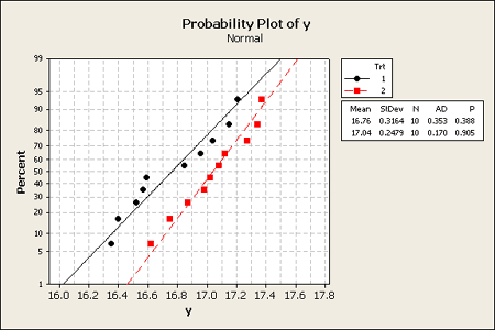
Normal probability plots look reasonable.

Confidence intervals involve finding an interval, in this case, the interval is about the difference in means. We want to find upper and lower limits that include the true difference in the means with a specified level of confidence, typically we will use 95%.
In the cases where we have a two-sided hypothesis test which rejects the null hypothesis, then the confidence interval will not contain 0. In our example above we can see in the Minitab output that the 95% confidence interval does not include the value 0, the hypothesized value for the difference, when the null hypothesis assumes the two means are equal.