Lesson 3 is the beginning of the one-way analysis of variance part of the course, which extends the two sample situation to k samples..
Text Reading: In addition to these notes, read Chapter 3 of the text and the online supplement. (If you have the 7th edition, also read 13.1.)
We review the issues related to a single factor experiment, which we see in the context of a Completely Randomized Design (CRD). In a single factor experiment with a CRD, the levels of the factor are randomly assigned to the experimental units. Alternatively, we can think of randomly assigning the experimental units to the treatments or in some cases, randomly selecting experimental units from each level of the factor.
Example 3-1: Cotton Tensile Strength Section

This is an investigation into the formulation of synthetic fibers that are used to make cloth. The response is tensile strength, the strength of the fiber. The experimenter wants to determine the best level of the cotton in terms of percent, to achieve the highest tensile strength of the fiber. Therefore, we have a single quantitative factor, the percent of cotton combined with synthetic fabric fibers.
The five treatment levels of percent cotton are evenly spaced from 15% to 35%. We have five replicates, five runs on each of the five cotton weight percentages.
| Cotton Weight Percentage |
Observations | ||||||
|---|---|---|---|---|---|---|---|
| 1 | 2 | 3 | 4 | 5 | Total | Average | |
| 15 | 7 | 7 | 15 | 11 | 9 | 49 | 9.8 |
| 20 | 12 | 17 | 12 | 18 | 18 | 77 | 15.4 |
| 25 | 14 | 18 | 18 | 19 | 19 | 88 | 17.6 |
| 30 | 19 | 25 | 22 | 19 | 23 | 108 | 21.6 |
| 35 | 7 | 10 | 11 | 15 | 11 | 54 | 10.8 |
| 376 | 15.04 | ||||||
The box plot of the results shows an indication that there is an increase in strength as you increase the cotton and then it seems to drop off rather dramatically after 30%.

Makes you wonder about all of those 50% cotton shirts that you buy?!
The null hypothesis asks: does the cotton percent make a difference? Now, it seems that it doesn't take statistics to answer this question. All we have to do is look at the side by side box plots of the data and there appears to be a difference – however, this difference is not so obvious by looking at the table of raw data. A second question, frequently asked when the factor is quantitative: what is the optimal level of cotton if you only want to consider strength?
There is a point that I probably should emphasize now and repeatedly throughout this course. There is often more than one response measurement that is of interest. You need to think about multiple responses in any given experiment. In this experiment, for some reason, we are interested in only one response, tensile strength, whereas in practice the manufacturer would also consider comfort, ductility, cost, etc.
This single factor experiment can be described as a completely randomized design (CRD). The completely randomized design means there is no structure among the experimental units. There are 25 runs which differ only in the percent cotton, and these will be done in random order. If there were different machines or operators, or other factors such as the order or batches of material, this would need to be taken into account. We will talk about these kinds of designs later. This is an example of a completely randomized design where there are no other factors that we are interested in other than the treatment factor percentage of cotton.
Reference: Problem 3.10 of Montgomery (3.8 in the \(7^{th}\) edition)
Analysis of Variance Section
The Analysis of Variance (ANOVA) is a somewhat misleading name for this procedure. But we call it the analysis of variance because we are partitioning the total variation in the response measurements.
The Model Statement
Each measured response can be written as the overall mean plus the treatment effect plus a random error.
\(Y_{ij} = \mu + \tau_i +\epsilon_{ij}\)
\(i = 1, ... , a,\) and \( j = 1, ... n_i\)
Generally, we will define our treatment effects so that they sum to 0, a constraint on our definition of our parameters,\(\sum \tau_{i}=0\). This is not the only constraint we could choose, one treatment level could be a reference such as the zero level for cotton and then everything else would be a deviation from that. However, generally, we will let the effects sum to 0. The experimental error terms are assumed to be normally distributed, with zero mean and if the experiment has constant variance then there is a single variance parameter \(\sigma^2\). All of these assumptions need to be checked. This is called the effects model.
An alternative way to write the model, besides the effects model, where the expected value of our observation, \(E\left(Y_{i j}\right)=\mu+\tau_{i}\) or an overall mean plus the treatment effect. This is called the means model and is written as:
\(Y_{ij} = \mu +\epsilon_{ij}\)
\(i = 1, ... , a,\) and \( j = 1, ... n_i\)
In looking ahead there is also the regression model. Regression models can also be employed but for now, we consider the traditional analysis of variance model and focus on the effects of the treatment.
Analysis of variance formulas that you should be familiar with by now are provided in the textbook.
The total variation is the sum of the observations minus the overall mean squared, summed over all a × n observations.
The analysis of variance simply takes this total variation and partitions it into the treatment component and the error component. The treatment component is the difference between the treatment mean and the overall mean. The error component is the difference between the observations and the treatment mean, i.e. the variation not explained by the treatments.
Notice when you square the deviations there are also cross-product terms, (see equation 3-5), but these sum to zero when you sum over the set of observations. The analysis of variance is the partition of the total variation into treatment and error components. We want to test the hypothesis that the means are equal versus at least one is different, i.e.
\(H_0 \colon \mu_{1}=\ldots=\mu_{a}\) versus \(H_a \colon \mu_{i} \neq \mu_{i'}\)
Corresponding to the sum of squares (SS) are the degrees of freedom associated with the treatments, \(a - 1\), and the degrees of freedom associated with the error, \(a × (n - 1)\), and finally one degree of freedom is due to the overall mean parameter. These add up to the total \(N = a × n\), when the \(n_i\) are all equal to \(n\), or \( N=\sum n_{i}\) otherwise.
The mean square treatment (MST) is the sum of squares due to treatment divided by its degrees of freedom.
The mean square error (MSE) is the sum of squares due to error divided by its degrees of freedom.
If the true treatment means are equal to each other, i.e. the \(\mu_i\) are all equal, then these two quantities should have the same expectation. If they are different then the treatment component, MST will be larger. This is the basis for the F-test.
The basic test statistic for testing the hypothesis that the means are all equal is the F ratio, MST/MSE, with degrees of freedom, a-1, and a×(n-1) or a-1 and N-a.
We reject \(H_0\) if this quantity is greater than \(1-α\) percentile of the F distribution.
Example 3-1: Continued - Cotton Weight Percent Section
Here is the Analysis of Variance table from the Minitab output:
One-way ANOVA: Observations versus Cotton Weight %
| Source | DF | SS | MS | F | P |
|---|---|---|---|---|---|
| Cotton Weight % | 4 | 475.76 | 118.94 | 14.76 | 0.000 |
| Error | 20 | 161.20 | 8.06 | ||
| Total | 24 | 636.96 |
| S = 2.839 | R-Sq = 74.69% | R-Sq(adj)=69.63% |
Individual 95% CIs for Mean based on Pooled StDev
| Level | N | Mean | StDev | ------+----------+----------+----------+--- |
|---|---|---|---|---|
| 15 | 5 | 9.800 | 3.347 | (-----*-----) |
| 20 | 5 | 15.400 | 3.130 | (----*----) |
| 25 | 5 | 17.600 | 2.074 | (----*----) |
| 30 | 5 | 21.600 | 2.608 | (----*----) |
| 35 | 5 | 10.800 | 2.864 | (-----*----) |
| ------+----------+----------+----------+--- | ||||
| 10.0 15.0 20.0 25.0 | ||||
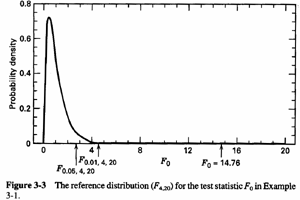
Note a very large F statistic that is, 14.76. The p-value for this F-statistic is < .0005 which is taken from an F distribution pictured below with 4 and 20 degrees of freedom.

We can see that most of the distribution lies between zero and about four. Our statistic, 14.76, is far out in the tail, obvious confirmation about what the data show, that indeed the means are not the same. Hence, we reject the null hypothesis.
Model Assumption Checking Section
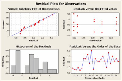
We should check if the data are normal - they should be approximately normal - they should certainly have constant variance among the groups. Independence is harder to check but plotting the residuals in the order in which the operations are done can sometimes detect if there is lack of independence. The question, in general, is how do we fit the right model to represent the data observed. In this case, there's not too much that can go wrong since we only have one factor and it is a completely randomized design. It is hard to argue with this model.
Let's examine the residuals, which are just the observations minus the predicted values, in this case, treatment means. Hence, \(e_{ij}=y_{ij}-\bar{y}_{i}\).

These plots don't look exactly normal but at least they don't seem to have any wild outliers. The normal scores plot looks reasonable. The residuals versus the order of the data plot are a plot of the error residuals data in the order in which the observations were taken. This looks a little suspect in that the first six data points all have small negative residuals which are not reflected in the following data points. Does this look like it might be a startup problem? These are the kinds of clues that you look for... if you are conducting this experiment you would certainly want to find out what was happening in the beginning.
Post-ANOVA Comparison of Means Section
So, we found the means are significantly different. Now what? In general, if we had a qualitative factor rather than a quantitative factor we would want to know which means differ from which other ones. We would probably want to do t-tests or Tukey maximum range comparisons, or some set of contrasts to examine the differences in means. There are many multiple comparison procedures.
Two methods, in particular, are Fisher's Least Significant Difference (LSD), and the Bonferroni Method. Both of these are based on the t-test. Fisher's LSD says do an F-test first and if you reject the null hypothesis, then just do ordinary t-tests between all pairs of means. The Bonferroni method is similar but only requires that you decide in advance how many pairs of means you wish to compare, say g, and then perform the g t-tests with a type I level of \(\alpha / g\). This provides protection for the entire family of g tests that the type I error is no more than \(\alpha \). For this setting, with a treatments, g = a(a-1)/2 when comparing all pairs of treatments.
All of these multiple comparison procedures are simply aimed at interpreting or understanding the overall F-test --which means are different? They apply to many situations especially when the factor is qualitative. However, in this case, since cotton percent is a quantitative factor, doing a test between two arbitrary levels e.g. 15% and 20% level, isn't really what you want to know. What you should focus on is the whole response function as you increase the level of the quantitative factor, cotton percent.
Whenever you have a quantitative factor you should be thinking about modeling that relationship with a regression function.
Review the video that demonstrates the use of polynomial regression to help explain what is going on.
Here is the Minitab output where regression was applied:
Polynomial Regression Analysis: Observation versus Cotton Weight %
The regression equations is:
Observations = 62.61 - 9.011 Cotton Weight % + 0.4814 cotton Weight % **2 - 0.007600 Cotton Weight%**3
| S = 3.04839 | R-Sq = 69.4% | R-Sq(sq) = 65.0% |
Analysis of Variance
| Source | DF | SS | MS | F | P |
| Regression | 3 | 441.814 | 147.271 | 15.85 | 0.000 |
| Error | 21 | 195.146 | 9.293 | ||
| Total | 24 | 636.960 |
Sequential Analysis of Variance
| Source | DF | SS | F | P |
| Linear | 1 | 33.620 | 1.28 | 0.269 |
| Quadratic | 1 | 343.214 | 29.03 | 0.000 |
| Cubic | 1 | 64.980 | 6.99 | 0.015 |
Here is a link to the Cotton Weight % dataset (cotton_weight.mwx | cotton_weight.csv). Open this in Minitab so that you can try this yourself.
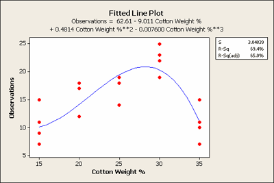
You can see that the linear term in the regression model is not significant but the quadratic is highly significant. Even the cubic term is significant with p-value = 0.015. In Minitab we can plot this relationship in the fitted line plot as seen below:

This shows the actual fitted equation. Why wasn't the linear term significant? If you just fit a straight line to this data it would be almost flat, not quite but almost. As a result, the linear term by itself is not significant. We should still leave it in the polynomial regression model, however, because we like to have a hierarchical model when fitting polynomials. What we can learn from this model is that the tensile strength of cotton is probably best between the 25 and 30 weight.
This is a more focused conclusion than we get from simply comparing the means of the actual levels in the experiment because the polynomial model reflects the quantitative relationship between the treatment and the response.
We should also check whether the observations have constant variance \(\sigma^2\), for all treatments. If they are all equal we can say that they are equal to \(\sigma^2\). This is an assumption of the analysis and we need to confirm this assumption. We can either test it with Bartlett's test, the Levene's test, or simply use the 'eye ball' technique of plotting the residuals versus the fitted values and see if they are roughly equal. The eyeball approach is almost as good as using these tests since by testing we cannot ‘prove’ the null hypothesis.
Bartlett's test is very susceptible to non-normality because it is based on the sample variances, which are not robust to outliers. We must assume that the data are normally distributed and thus not very long-tailed. When one of the residuals is large and you square it, you get a very large value which explains why the sample variance is not very robust. One or two outliers can cause any particular variance to be very large. Thus simply looking at the data in a box plot is as good as these formal tests. If there is an outlier you can see it. If the distribution has a strange shape you can also see this in a histogram or a box plot. The graphical view is very useful in this regard.
Levene's test is preferred to Bartlett’s in my view because it is more robust. To calculate the Levene's test you take the observations and obtain (not the squared deviations from the mean but) the absolute deviations from the median. Then, you simply do the usual one way ANOVA F-test on these absolute deviations from the medians. This is a very clever and simple test that has been around for a long time, created by Levene back in the 1950s. It is much more robust to outliers and non-normality than Bartlett's test.