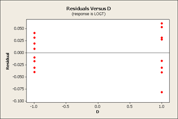
When you look at the graph of the residuals as shown below you can see that the variance is small at the low end and the variance is quite large on the right side producing a fanning effect. Consider the family of transformations that can be applied to the response \(y_{ij}\).
Transformations towards the bottom of the list are stronger in how they shrink large values more than they shrink small values that are represented on the plot. This pattern of the residuals is one clue to get you to be thinking about the type of transformations you would select.
The other consideration and thinking about transformations of the response \(y_{ij}\) is what it does to the relationship itself. Some of you will recall from other classes the Tukey one-degree-of-freedom test for interaction. This is a test for interaction where you have one observation per cell such as with a randomized complete block design. But with one observation per cell and two treatments our model would be :
\(Y_{ijk}= \mu+\alpha_{i}+\beta_{j}+(\alpha\beta)_{ij}+\epsilon_{ijk}\)
where,
i = 1 ... a,
j = 1 ... b, with
k = 1 ... 1, (only have one observation per cell)
There is no estimate of pure error so we cannot fit the old model. The model proposed by Tukey's has one new parameter (γ) gamma :
\(Y_{ij}= \mu+\alpha_{i}+\beta_{j}+\gamma\alpha_{i}\beta_{j}+\epsilon_{ij}\)
This single parameter, gamma, is the 1 degree of freedom term and so our error,\(\epsilon_{ij}\), has (a-1)(b-1) -1 degrees of freedom. This model allows for just a single additional parameter which is based on a multiplicative effect on the two factors.
Now, when is this applicable?
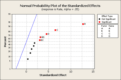
Let's go back to the drill rate example (Ex6-3.MTW | Ex6-3.csv) where we saw the fanning effect in the plot of the residuals. In this example B, C and D were the three main effects and there were two interactions BD and BC. From Minitab we can reproduce the normal probability plot for the full model.
But let's first take a look at the residuals versus our main effects B, C and D.
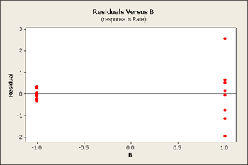
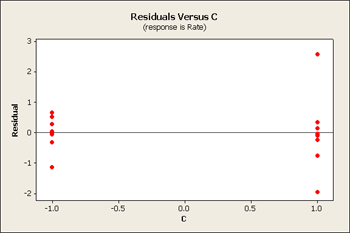
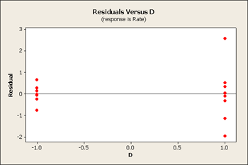
All three of these residuals versus the main effects show same pattern, the large predicted values tend to have larger variation.
Next, what we really want to look at is the factorial plots for these three factors, B, C and D and the interactions among these, BD and BC.
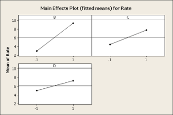
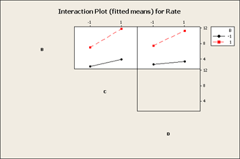
What you see in the interaction plot above is a pattern that is non-parallel showing there is interaction present. But, from what you see in the residual graph what would you expect to see on this factor plot?
The tell-tale pattern that is useful here is an interaction that does not have crossing lines - a fanning effect - and it is exactly the same pattern that allows the Tukey model to fit. In both cases, it is a pattern of interaction that you can remove by transformation. If we select a transformation that will shrink the large values more than it does the small values and the overall result would be that we would see less of this fan effect in the residuals.
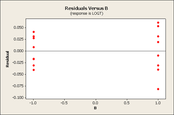
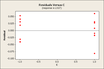
We can look at either the square root or log transformation. It turns out that the log transformation is the one that seems to fit the best. On a log scale it looks somewhat better - it might not be perfect but it is certainly better than what we had before.
Let's also look at the analysis of variance.
Factorial Fit: LOGT versus B, C, D
Estimated Effects and Coefficients for LOGT (coded units)
| Term | Effect | Coef | SE Coef | T | P |
|---|---|---|---|---|---|
| Constant | 0.69355 | 0.01218 | 56.94 | 0.000 | |
| B | 0.50204 | 0.25102 | 0.01218 | 20.61 | 0.000 |
| C | 0.25126 | 0.12563 | 0.01218 | 10.31 | 0.000 |
| D | 0.14248 | 0.07124 | 0.01218 | 5.85 | 0.000 |
| B*C | -0.02114 | -0.01057 | 0.01218 | -0.87 | 0.406 |
| B*D | 0.04196 | 0.02098 | 0.01218 | 1.72 | 0.116 |
| S = 0.0487213 R-Sq = 98.27% R-Sq(adj) = 97.41% | |||||
Analysis of Variance for LOGT (coded units)
| Source | DF | Seq SS | Adj SS | Adj MS | F | P |
|---|---|---|---|---|---|---|
| Main Effects | 3 | 1.34190 | 1.34190 | 0.447300 | 188.44 | 0.000 |
| 2-Way Interactions | 2 | 0.00883 | 0.00883 | 0.004414 | 1.86 | 0.206 |
| Residual Error | 10 | 0.02374 | 0.02374 | 0.002374 | ||
| Lack of Fit | 2 | 0.00112 | 0.00112 | 0.000558 | 0.20 | 0.825 |
| Pure Error | 8 | 0.02262 | 0.02262 | 0.002828 | ||
| Total | 15 | 1.37447 | ||||
The overall main effects are still significant. But the two 2-way interactions effects combined are no longer significant, and individually, the interactions are not significant here either. So, the log transformation which improved the unequal variances pulled the higher responses down more than the lower values and therefore resulted in more of a parallel shape. What's good for variance is good for a simple model. Now we are in a position where we can drop the interactions and reduce this model to a main effects only model.
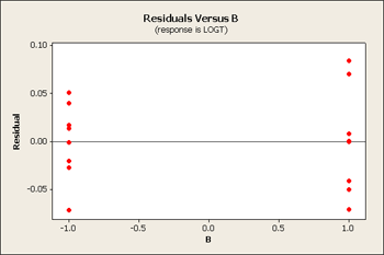
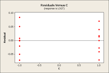
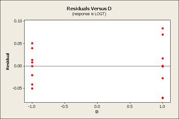
Now our residual plots are nearly homoscedastic for B, C and D. See below...
Serendipity - good things come in packages! When you pick the correct transformation, you sometimes achieve constant variance and a simpler model.
Many times you can find a transformation that will work for your data - giving you a simpler analysis but it doesn't always work.
Transformations are typically performed to:
- Stabilize variance - to achieve equal variance
- Improve normality - this is often violated because it is easy to have an outlier when variance is large which can be 'reined in' with a transformation
- Simplify the model
Sometimes transformations will solve a couple of these problems.
Is there always a transformation that can be applied to equalize variance? Not really ... there are two approaches to solving this question. First, we could use some non-parametric method. Although non-parametric methods have fewer assumptions about the distribution, you still have to worry about how you are measuring the center of the distribution. When you have a non-parametric situation you may have a different shaped distribution in different parts of the experiment. You have to be careful about using the mean in one case, and the media in another ... but that is one approach.
The other approach is a weighted analysis, where you weight the observations according to the inverse of their variance. There are situations where you have unequal variation for maybe a known reason or unknown reason, but if you have repeated observations and you can get weights, then you can do a weighted analysis.
It is this course author's experience many times you can find a transformation when you have this kind of pattern. Also, sometimes when you have unequal variance you just have a couple of bad outliers, especially when you only have one or a few observations per cell. In this case it is difficult to the distinguish whether you have a couple of outliers or the data is heteroscedastic - it is not always clear.
Empirical Selection of Lambda Section
Prior (theoretical) knowledge or experience can often suggest the form of a transformation. However, another method for the analytical selection of lambda for the exponent used in the transformation is the Box-Cox (1964). This method simultaneously estimates the model parameters and the transformation parameter lambda.
Box-Cox method is implemented in some statistical software applications.
Example 6.4 Section
This example is a four-factor design in a manufacturing situation where injection molding is the focus. Injection molding is a very common application in the industry; a \(2^k\) design where you have many factors influencing the quality which is measured by how many defects are created by the process. Almost anything that you can think of which has been made out of plastic was created through the injection molding process.
See the example in (Ex6-4.mwx | Ex6-4.csv)
In this example we have four factors again: A = temperature of the material, B = clamp time for drying, C = resin flow, and D = closing time of the press. What we are measuring as the response is number of defects. This is recorded as an index of quality in terms of percent. As you look through the data in Figure 6.29 (7th edition) you can see percent of defects as high as 15.5% or as low as 0.5%. Let's analyze the full model in Minitab.
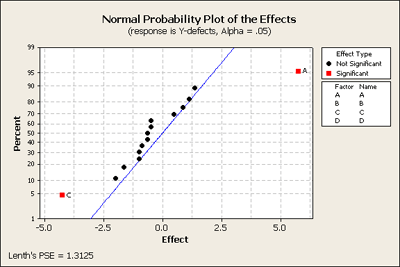
The normal probability plot of the effects shows us that two of the factors A and C are both significant and none of the two-way interactions are significant.
What we want to do next is look at the residuals vs. variables A, B, C, D in a reduced model with just the main effects as none of the interactions seemed important.
For each factor, you see that the residuals are more dispersed (higher variance) to the right than to the left. Overall, however, the residuals do not look too bad and the normal plot also does not look too bad. When we look at the p-values we find that A and C are significant but B and D are not.
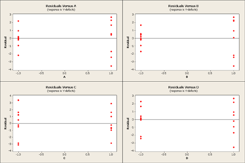
But there is something else that can be learned here. The point of this example is that although the B factor is not significant as it relates to the response, percentage of product defects - however if you are looking for a recommended setting for B you should use the low level for B. A and C, are significant and will reduce the number of defects. However, by choosing B at the low level you will produce a more homogeneous product, products with less variability. What is important in product manufacturing is not only reducing the number of defects but also producing products that are uniform. This is a secondary consideration that should be taken into account after the primary considerations related to the percent of product defects.