Example 4.1: Vascular Graft Section
This example investigates a procedure to create artificial arteries using a resin. The resin is pressed or extruded through an aperture that forms the resin into a tube.
To conduct this experiment as a RCBD, we need to assign all 4 pressures at random to each of the 6 batches of resin. Each batch of resin is called a “block”, since a batch is a more homogenous set of experimental units on which to test the extrusion pressures. Below is a table which provides percentages of those products that met the specifications.
| Extrusion Pressure (PSI) | Batch of Resin (Block) | Treatment Total | |||||
|---|---|---|---|---|---|---|---|
| 1 | 2 | 3 | 4 | 5 | 6 | ||
| 8500 | 90.3 | 89.2 | 98.2 | 93.9 | 87.4 | 97.9 | 556.9 |
| 8700 | 92.5 | 89.5 | 90.6 | 94.7 | 87.0 | 95.8 | 550.1 |
| 8900 | 85.5 | 90.8 | 89.6 | 86.2 | 88.0 | 93.4 | 533.5 |
| 9100 | 82.5 | 89.5 | 85.6 | 87.4 | 78.9 | 90.7 | 514.6 |
| Block Totals | 350.8 | 359.0 | 364.0 | 362.2 | 341.3 | 377.8 | \(y_n = 2155.1\) |
| Table 4-3 Randomized Complete Block Design for the Vascular Graft Experiment | |||||||
Output...
Response: Yield
ANOVA for selected Factorial Model
Analysis of variance table [Partial sum of squares]
| Source | Sum of Squares | DF | Mean Square | F Value | Prob > F |
|---|---|---|---|---|---|
| Block | 192.25 | 5 | 38.45 | ||
| Model | 178.17 | 3 | 59.39 | 8.11 | 0.0019 |
| A | 178.17 | 3 | 59.39 | 8.11 | 0.0019 |
| Residual | 109.89 | 15 | 7.33 | ||
| Cor Total | 480.31 | 23 |
| Std. Dev. | 2.71 | R-Squared | 0.6185 |
| Mean | 89.80 | Adj R-Squared | 0.5422 |
| C.V. | 3.01 | Pred R-Squared | 0.0234 |
| PRESS | 281.31 | Adeq Precision | 9.759 |
Notice that Design Expert does not perform the hypothesis test on the block factor. Should we test the block factor?
Below is the Minitab output which treats both batch and treatment the same and tests the hypothesis of no effect.
ANOVA: Yield versus Batch, Pressure
| Factor | Type | Level | Values |
|---|---|---|---|
| Batch | random | 6 | 1,2,3,4,5,6 |
| Pressure | fixed | 4 | 8500, 8700, 8900, 9100 |
Analysis of Variance for Yield
| Source | DF | SS | MS | F | P |
|---|---|---|---|---|---|
| Batch | 5 | 192.252 | 38.450 | 5.25 | 0.006 |
| Pressure | 3 | 178.171 | 59.390 | 8.11 | 0.002 |
| Error | 15 | 109.886 | 7.326 | ||
| Total | 23 | 480.310 |
| S = 2.70661 | R-Sq = 77.12% | R-Sq(adj) = 64.92% |
This example shows the output from the ANOVA command in Minitab (Menu > Stat > ANOVA > Balanced ANOVA). It does hypothesis tests for both batch and pressure, and they are both significant. Otherwise, the results from both programs are very similar.
Again, should we test the block factor? Generally, the answer is no, but in some instances, this might be helpful. We use the RCBD design because we hope to remove from error the variation due to the block. If the block factor is not significant, then the block variation, or mean square due to the block treatments is no greater than the mean square due to the error. In other words, if the block F ratio is close to 1 (or generally not greater than 2), you have wasted effort in doing the experiment as a block design, and used in this case 5 degrees of freedom that could be part of error degrees of freedom, hence the design could actually be less efficient!
Therefore, one can test the block simply to confirm that the block factor is effective and explains variation that would otherwise be part of your experimental error. However, you generally cannot make any stronger conclusions from the test on a block factor, because you may not have randomly selected the blocks from any population, nor randomly assigned the levels.
Why did I first say no?
There are two cases we should consider separately when blocks are: 1) a classification factor and 2) an experimental factor. In the case where blocks are a batch, it is a classification factor, but it might also be subjects or plots of land which are also classification factors. For a RCBD you can apply your experiment to convenient subjects. In the general case of classification factors, you should sample from the population in order to make inferences about that population. These observed batches are not necessarily a sample from any population. If you want to make inferences about a factor then there should be an appropriate randomization, i.e. random selection, so that you can make inferences about the population. In the case of experimental factors, such as oven temperature for a process, all you want is a representative set of temperatures such that the treatment is given under homogeneous conditions. The point is that we set the temperature once in each block; we don't reset it for each observation. So, there is no replication of the block factor. We do our randomization of treatments within a block. In this case, there is an asymmetry between treatment and block factors. In summary, you are only including the block factor to reduce the error variation due to this nuisance factor, not to test the effect of this factor.
ANOVA: Yield versus Batch, Pressure Section
The residual analysis for the Vascular Graft example is shown:
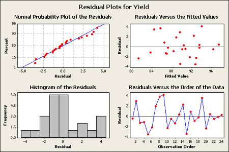
The pattern does not strike me as indicating an unequal variance.
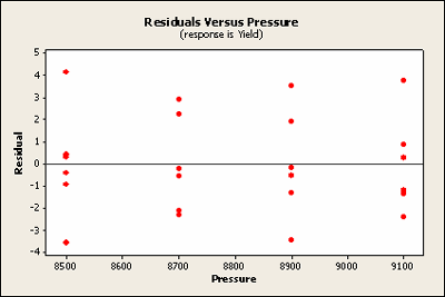
Another way to look at these residuals is to plot the residuals against the two factors. Notice that pressure is the treatment factor and batch is the block factor. Here we'll check for homogeneous variance. Against treatment these look quite homogeneous.
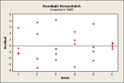
Plotted against block the sixth does raise ones eyebrow a bit. It seems to be very close to zero.
Basic residual plots indicate that normality, constant variance assumptions are satisfied. Therefore, there seems to be no obvious problems with randomization. These plots provide more information about the constant variance assumption, and can reveal possible outliers. The plot of residuals versus order sometimes indicates a problem with the independence assumption.
Missing Data Section
In the example dataset above, what if the data point 94.7 (second treatment, fourth block) was missing? What data point can I substitute for the missing point?
If this point is missing we can substitute x, calculate the sum of squares residuals, and solve for x which minimizes the error and gives us a point based on all the other data and the two-way model. We sometimes call this an imputed point, where you use the least squares approach to estimate this missing data point.
After calculating x, you could substitute the estimated data point and repeat your analysis. Now you have an artificial point with known residual zero. So you can analyze the resulting data, but now should reduce your error degrees of freedom by one. In any event, these are all approximate methods, i.e., using the best fitting or imputed point.
Before high-speed computing, data imputation was often done because the ANOVA computations are more readily done using a balanced design. There are times where imputation is still helpful but in the case of a two-way or multiway ANOVA we generally will use the General Linear Model (GLM) and use the full and reduced model approach to do the appropriate test. This is often called the General Linear Test (GLT).
Let's take a look at this in Minitab now (no sound)...
The sum of squares you want to use to test your hypothesis will be based on the adjusted treatment sum of squares, \(R( \tau_i | \mu, \beta_j) \) using the notation for testing:
\(H_0 \colon \tau_i = 0\)
The numerator of the F-test, for the hypothesis you want to test, should be based on the adjusted SS's that is last in the sequence or is obtained from the adjusted sums of squares. That will be very close to what you would get using the approximate method we mentioned earlier. The general linear test is the most powerful test for this type of situation with unbalanced data.
The General Linear Test can be used to test for significance of multiple parameters of the model at the same time. Generally, the significance of all those parameters which are in the Full model but are not included in the Reduced model are tested, simultaneously. The F test statistic is defined as
\(F^\ast=\dfrac{SSE(R)-SSE(F)}{df_R-df_F}\div \dfrac{SSE(F)}{df_F}\)
Where F stands for “Full” and R stands for “Reduced.” The numerator and denominator degrees of freedom for the F statistic is \(df_R - df_F\) and \(df_F\) , respectively.
Here are the results for the GLM with all the data intact. There are 23 degrees of freedom total here so this is based on the full set of 24 observations.
General Linear Model: Yield versus, Batch, Pressure
| Factor | Type | Levels | Values |
|---|---|---|---|
| Batch | fixed | 6 | 1, 2, 3, 4, 5, 6 |
| Pressure | fixed | 4 | 8500, 8700, 8900, 9100 |
Analysis of variance for Yield, using Adjusted SS for Tests
| Source | DF | Seq SS | Adj SS | Adj MS | F | P |
|---|---|---|---|---|---|---|
| Batch | 5 | 192.252 | 192.252 | 38.450 | 5.25 | 0.006 |
| Pressure | 3 | 178.171 | 178.171 | 59.390 | 8.11 | 0.002 |
| Error | 15 | 109.886 | 109.886 | 7.326 | ||
| Total | 23 | 480.310 |
| S = 2.70661 | R-Sq = 77.12% | R-Sq(adj) =64.92% |
Least Squares Means for Yield
| Pressure | Mean | SE Mean | |
|---|---|---|---|
| 8500 | 92.82 | 1.105 | |
| 8700 | 91.68 | 1.105 | |
| 8900 | 88.92 | 1.105 | |
| 9100 | 85.77 | 1.105 | |
| Main Effects Plot (fitted means) for Yield | |||
When the data are complete this analysis from GLM is correct and equivalent to the results from the two-way command in Minitab. When you have missing data, the raw marginal means are wrong. What if the missing data point were from a very high measuring block? It would reduce the overall effect of that treatment, and the estimated treatment mean would be biased.
Above you have the least squares means that correspond exactly to the simple means from the earlier analysis.
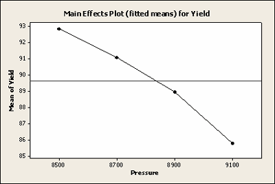
We now illustrate the GLM analysis based on the missing data situation - one observation missing (Batch 4, pressure 2 data point removed). The least squares means as you can see (below) are slightly different, for pressure 8700. What you also want to notice is the standard error of these means, i.e., the S.E., for the second treatment is slightly larger. The fact that you are missing a point is reflected in the estimate of error. You do not have as many data points on that particular treatment.
Results for: Ex4-1miss.MTW
General Linear Model: Yield versus, Batch, Pressure
| Factor | Type | Levels | Values |
|---|---|---|---|
| Batch | fixed | 6 | 1, 2, 3, 4, 5, 6 |
| Pressure | fixed | 4 | 8500, 8700, 8900, 9100 |
Analysis of variance for Yield, using Adjusted SS for Tests
| Source | DF | Seq SS | Adj SS | Adj MS | F | P |
|---|---|---|---|---|---|---|
| Batch | 5 | 190.119 | 189.522 | 37.904 | 5.22 | 0.007 |
| Pressure | 3 | 163.398 | 163.398 | 54.466 | 7.50 | 0.003 |
| Error | 14 | 101.696 | 101.696 | 7.264 | ||
| Total | 22 | 455.213 |
| S = 2.69518 | R-Sq = 77.66% | R-Sq(adj) =64.99% |
Least Squares Means for Yield
| Pressure | Mean | SE Mean |
|---|---|---|
| 8500 | 92.82 | 1.100 |
| 8700 | 91.08 | 1.238 |
| 8900 | 88.92 | 1.100 |
| 9100 | 85.77 | 1.100 |
The overall results are similar. We have only lost one point and our hypothesis test is still significant, with a p-value of 0.003 rather than 0.002.
Here is a plot of the least squares means for Yield with all of the observations included.
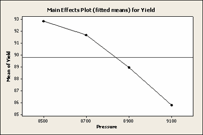
Here is a plot of the least squares means for Yield with the missing data, not very different.
Again, for any unbalanced data situation, we will use the GLM. For most of our examples, GLM will be a useful tool for analyzing and getting the analysis of variance summary table. Even if you are unsure whether your data are orthogonal, one way to check if you simply made a mistake in entering your data is by checking whether the sequential sums of squares agree with the adjusted sums of squares.