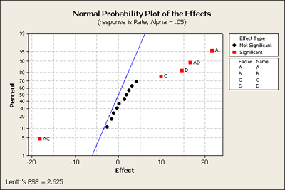
We discussed designing experiments, but now let's discuss how we would analyze these experiments. We take an example we saw before. The response Y is filtration rate in a chemical pilot plant and the four factors are: A = temperature, B = pressure, C = concentration and D = stirring rate. (Example 2 from Chapter 6, Ex6-2.mwx | Ex6-2.csv)
This experimental design has 16 observations, a \(2^4\) with one complete replicate. This is the example we looked at with one observation per cell when we introduced a normal scores plot.

Our final model ended up with three factors, A, C and D, and two of their interactions, AC and AD. This was based on one complete replicate of this design. What might we have learned if we had done an experiment half this size, N = 8? If we look at the fractional factorial - one half of this design - where we have D = ABC or I = ABCD as the generator - this creates a design with 8 observations.
Fractional Factorial Design
| Factors: | 4 | Base Design: | 4, 8 | Resolution: | IV |
| Runs: | 8 | Replicates: | 1 | Fraction: | 1/2 |
| Blocks: | 1 | Center pts (total): | 0 | ||
Design Generators: D = ABC
Alias Structure
I + ABCD
A + BCD
B + ACD
C + ABD
D + ABC
AB + CD
AC + BD
AD + BC
The alias structure is a four letter word, therefore this is a Resolution IV design, A, B, C and D are each aliased with a 3-way interaction, (so we can't estimate them any longer), and the two way interactions are aliased with each other.
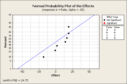
If we look at the analysis of this 1/2 fractional factorial design and we put all of the terms in the model, (of course some of these are aliased with each other), and we will look at the normal scores plot. What do we get? (The data are in Ex6_2Half.MTW)

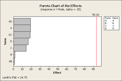
We only get seven effects plotted, since there were eight observations. The overall mean does not show up here. These points are labeled but because there are only seven of them there is no estimate of error. Let's look at another plot that we haven't used that much yet - the Pareto plot. This type of plot looks at the effects and orders them from largest to smallest showing you the relative sizes of the effects. Although we do not know what is significant and what is not significant, this still might be a helpful plot to look at to better understand the data.

This Pareto plot shows us that the three main effects A, C, and D that were most significant in the full design are still important as well as the two interactions, AD and AC. However, B and AB are clearly not as large. (You can do this using the Stat > DOE > Factorial > Analyze and click on Graph.)
What can we learn from this? Let's try to fit a reduced model from the information that we gleaned from this first step. We will include all the main effects and the AC and AD interactions.
In the analysis, we have four main effects ...
Factorial Fit: Y-Rate versus A, B, C, D
Estimated Effects and Coefficients for Y-Rate (coded units)
| Term | Effect | Coef | SE Coef | T | P |
|---|---|---|---|---|---|
| Constant | 70.750 | 0.5000 | 141.50 | 0.004 | |
| A | 19.000 | 9.500 | 0.5000 | 19.00 | 0.033 |
| B | 1.500 | 0.750 | 0.5000 | 1.50 | 0.374 |
| C | 14.000 | 7.000 | 0.5000 | 14.00 | 0.045 |
| D | 16.500 | 8.250 | 0.5000 | 16.50 | 0.039 |
| A*C | -18.500 | -9.250 | 0.5000 | -18.50 | 0.034 |
| A*D | 19.000 | 9.500 | 0.5000 | 19.00 | 0.033 |
| S = 1.41421 R-Sq = 99.93% R-Sq(adj) = 99.54% | |||||
Analysis of Variance for Y-Rate (coded units)
| Source | DF | Seq SS | Adj SS | Adj MS | F | P |
|---|---|---|---|---|---|---|
| Main Effects | 4 | 1663.00 | 1663.00 | 415.750 | 207.88 | 0.052 |
| 2-Way Interactions | 2 | 1406.50 | 1406.50 | 703.250 | 351.63 | 0.038 |
| Residual Error | 1 | 2.00 | 2.00 | 2.000 | ||
| Total | 7 | 3071.50 | ||||
... overall they are almost significant, (.052), and the overall two-way interactions, (.038) but we only have one degree of freedom of error - so this makes this a very low-power test. However, this is the price that you would pay with a fractional factorial. If we look above at the individual effects, B as we saw on the plot appears to be not important, we have further evidence that we should drop this from the analysis.
Back to Minitab and let's drop the B term because it doesn't show up as a significant main effect nor as part of any of the interactions.
Factorial Fit: Y-Rate versus A, C, D
Estimated Effects and Coefficients for Y-Rate (coded units)
| Term | Effect | Coef | SE Coef | T | P |
|---|---|---|---|---|---|
| Constant | 70.750 | 0.6374 | 111.0 | 0.000 | |
| A | 19.000 | 9.500 | 0.6374 | 14.90 | 0.004 |
| C | 14.000 | 7.000 | 0.6374 | 10.98 | 0.008 |
| D | 16.500 | 8.250 | 0.6374 | 12.94 | 0.006 |
| A*C | -18.500 | -9.250 | 0.6374 | -14.51 | 0.005 |
| A*D | 19.000 | 9.500 | 0.6374 | 14.90 | 0.004 |
| S = 1.80278 R-Sq = 99.79% R-Sq(adj) = 99.26% | |||||
Analysis of Variance for Y-Rate (coded units)
| Source | DF | Seq SS | Adj SS | Adj MS | F | P |
|---|---|---|---|---|---|---|
| Main Effects | 3 | 1658.50 | 1658.50 | 552.833 | 170.10 | 0.006 |
| 2-Way Interactions | 2 | 1406.50 | 1406.50 | 703.250 | 216.38 | 0.005 |
| Residual Error | 2 | 6.50 | 6.50 | 3.250 | ||
| Total | 7 | 3071.50 | ||||
Now the overall main effects and 2-way interactions are significant. Residual error still only has 2 degrees of freedom, but this gives us an estimate at least and we can also look at the individual effects.
So, fractional factorials are useful when you hope or expect that not all of the factors are going to be significant. You are screening for factors to drop out of the study. In this example, we started with a \(2^{4 - 1}\) design but when we dropped B we ended up with a \(2^3\) design with 1 observation per cell.
This is a typical scenario, you begin by screening a large number of factors and end up with a smaller set. We still don't know much about the factors and this is still a pretty thin or weak design but it gives you the information that you need to take the next step. You can now do a more complete experiment on fewer factors.