
STAT 504: 10.1.3 - Example: General Social Survey Section
Cross-classification of respondents according to choice for the president in 1992 presidential election (Bush, Clinton, Perot) and political view on the 7 point scale (extremely liberal, liberal, slightly liberal, moderate, slightly conservative, conservative, extremely conservative).
Let's group the 7 point scale to 3 levels, and consider a 3 × 3 table:
|
Bush
|
Clinton
|
Perot
|
Total
|
|
| Liberal |
70
|
324
|
56
|
450
|
| Moderate |
195
|
332
|
101
|
628
|
| Conservative |
382
|
199
|
117
|
698
|
|
Total
|
647
|
855
|
274
|
1774
|
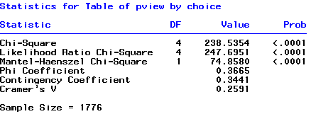
Are political view and choice independent? You already know how to do this with the chi-squared test of independence. For example, see /onlinecourses/sites/stat504/files/lesson05/vote.sas (output: vote.lst ) or vote.R., and compare the results of chi-squared tests with the log-linear model output.
Here is part of the output from SAS PROC FREQ ...
and a part from the output of the PROC GENMOD procedure.
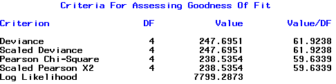
Question: Can you identify the X2 and G2 statistics in these two outputs? What is conclusion about independence? Does the model fit well or not? Can you identify the log-linear independence model and relevant part of the output? Note that if "Value/df" is much greater than 1, you have sufficient evidence to reject the model.
Here is what the log-linear model would be:
\(\text{log}(\mu_{ij})=\lambda+\lambda_i^{pview}+\lambda_j^{choice}\)
Recall, that we assume the counts are coming from a Poisson distribution and that all odds ratios are equal to 1. The explicit asumption is that the interaction term is equal to 0. Our null hypothesis is that the above specified loglinear model of independence fits versus the alternative that the saturated model fits.
What is the LR test statistic? Identify it in the PROC FREQ, PROC GENMOD and PROC CATMOD part of the output. Notice, that in GENMOD, "conservative" and "perot" are reference levels. Thus equation for each "Choice" is:
Bush: log(μi1) = λ + λipview + λ1choice
Clinton: log(μi2) = λ + λipview + λ2choice
Perot: log(μi3) = λ + λipview - λ1choice - λ2choice in CATMOD. Notice in GENMOD with dummy coding this would be: log(μi3) = λ + λipview +λ3choice
If we want, for example, probability of being a liberal and voting for Bush:
Lib-Bush: log(μ11) = λ + λ1pview + λ1choice =4.68-0.439+0.859
How about the odds? We would look at the difference of the above equations; also see the previous page on general set up of parameters. For example,
Bush-Clinton: λ + λipview + λ1choice - (λ + λipview + λ2choice) = λ1choice- λ2choice
Bush-Perot: 2 λ1choice+λ2choice in CATMOD. Notice in GENMOD with dummy coding this would be: λ1choice - λ3choice
Clinton-Perot: λ1choice+2 λ2choice in CATMOD. Notice in GENMOD with dummy coding this would be: λ2choice - λ3choice
Clinton has better odds!
CATMOD: \(\text{exp}(\lambda_1^B-\lambda_2^B)=\text{exp}(0.1935-0.4722)=0.756\)
GENMOD: \(\text{exp}(0.8592-1.1380)=0.756\)R, glm(): exp(pchoiceclinton)=exp(0.27876)=1.3215 which are the odds of Clinton vs. Bush, so Bush vs. Clinton is 1/1.3215=0.756
Think about it!How about Bush vs. Perot, e.g. 647/274?Bush has twice the odds of Perot of being picked for the presidency.
CATMOD: \(\text{exp}(2\lambda_1^B+\lambda_2^B)=\text{exp}(2\times 0.1935+0.4722)=2.361\)
GENMOD: \(\text{exp}(\lambda_1^B)=\text{exp}(0.8592)=2.361\)R, glm(): 1/exp(pchoiceperot)=exp(-pchoiceperot)=exp(0.86992)=2.361
asdasdasd
Here is the output from GENMOD in SAS. The highlighted row are the possible residulas values as we dicussed earlier. Let's look at the standardized Perason residulas; recall they have approximate N(0,1) distribution, so we are looking for the absolute values which are greater than 2 or 3. Notice, for example, for the first cell, the value is -10.649., clearly a large residuls. Look at the other cells.
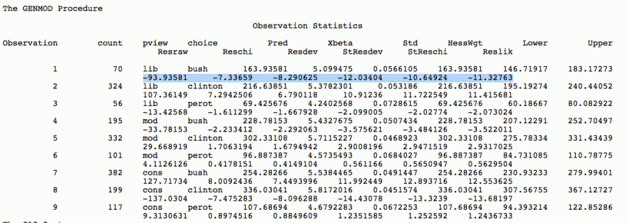
In R, glm() there are a number of ways to get the residuals, but one would be to use residuals() function, and to specify the type we want, e.g., the following code produces pearson residuals, the standardized (adjusted) residulas, with the formatted output. Notice the same values for the fist cell as we got from GENMOD above.
resids <- residuals(vote.ind,type="pearson")
h <- lm.influence(vote.ind)$hat
adjresids <- resids/sqrt(1-h)
round(cbind(count,fits,adjresids),2)

  count   fits adjresids
1    70 163.94    -10.65
2   324 216.64     11.72
3    56  69.43     -2.03
4   195 228.78     -3.48
5   332 302.33      2.95
6   101  96.89      0.57
7   382 254.28     12.89
8   199 336.03    -13.32
9   117 107.69      1.25