
Let's review the basic concept of a confidence interval.
Suppose we want to estimate an actual population mean \(\mu\). As you know, we can only obtain \(\bar{x}\), the mean of a sample randomly selected from the population of interest. We can use \(\bar{x}\) to find a range of values:
\[\text{Lower value} < \text{population mean}\;\; \mu < \text{Upper value}\]
that we can be really confident contains the population mean \(\mu\). The range of values is called a "confidence interval."
Example S.2.1
Should using a hand-held cell phone while driving be illegal? Section
There is little doubt that you have seen numerous confidence intervals for population proportions reported in newspapers over the years.
For example, a newspaper report (ABC News poll, May 16-20, 2001) was concerned about whether or not U.S. adults thought using a hand-held cell phone while driving should be illegal. Of the 1,027 U.S. adults randomly selected for participation in the poll, 69% believed it should be illegal. The reporter claimed that the poll's "margin of error" was 3%. Therefore, the confidence interval for the (unknown) population proportion p is 69% ± 3%. That is, we can be really confident that between 66% and 72% of all U.S. adults think using a hand-held cell phone while driving a car should be illegal.
General Form of (Most) Confidence Intervals Section
The previous example illustrates the general form of most confidence intervals, namely:
$\text{Sample estimate} \pm \text{margin of error}$
The lower limit is obtained by:
$\text{the lower limit L of the interval} = \text{estimate} - \text{margin of error}$
The upper limit is obtained by:
$\text{the upper limit U of the interval} = \text{estimate} + \text{margin of error}$
Once we've obtained the interval, we can claim that we are really confident that the value of the population parameter is somewhere between the value of L and the value of U.
So far, we've been very general in our discussion of the calculation and interpretation of confidence intervals. To be more specific about their use, let's consider a specific interval, namely the "t-interval for a population mean µ."
(1-α)100% t-interval for the population mean \(\mu\)
If we are interested in estimating a population mean \(\mu\), it is very likely that we would use the t-interval for a population mean \(\mu\).
- t-Interval for a Population Mean
- The formula for the confidence interval in words is:
$\text{Sample mean} \pm (\text{t-multiplier} \times \text{standard error})$
- and you might recall that the formula for the confidence interval in notation is:
- $\bar{x}\pm t_{\alpha/2, n-1}\left(\dfrac{s}{\sqrt{n}}\right)$
Note that:
- the "t-multiplier," which we denote as \(t_{\alpha/2, n-1}\), depends on the sample size through n - 1 (called the "degrees of freedom") and the confidence level \((1-\alpha)\times100%\) through \(\frac{\alpha}{2}\).
- the "standard error," which is \(\frac{s}{\sqrt{n}}\), quantifies how much the sample means \(\bar{x}\) vary from sample to sample. That is, the standard error is just another name for the estimated standard deviation of all the possible sample means.
- the quantity to the right of the ± sign, i.e., "t-multiplier × standard error," is just a more specific form of the margin of error. That is, the margin of error in estimating a population mean µ is calculated by multiplying the t-multiplier by the standard error of the sample mean.
- the formula is only appropriate if a certain assumption is met, namely that the data are normally distributed.
Clearly, the sample mean \(\bar{x}\), the sample standard deviation s, and the sample size n are all readily obtained from the sample data. Now, we need to review how to obtain the value of the t-multiplier, and we'll be all set.
How is the t-multiplier determined?
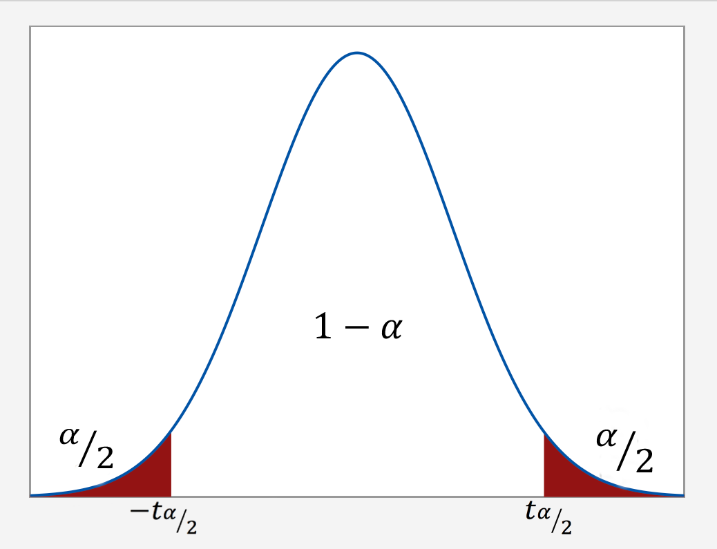
As the following graph illustrates, we put the confidence level $1-\alpha$ in the center of the t-distribution. Then, since the entire probability represented by the curve must equal 1, a probability of α must be shared equally among the two "tails" of the distribution. That is, the probability of the left tail is $\frac{\alpha}{2}$ and the probability of the right tail is $\frac{\alpha}{2}$. If we add up the probabilities of the various parts $(\frac{\alpha}{2} + 1-\alpha + \frac{\alpha}{2})$, we get 1. The t-multiplier, denoted \(t_{\alpha/2}\), is the t-value such that the probability "to the right of it" is $\frac{\alpha}{2}$:
It should be no surprise that we want to be as confident as possible when we estimate a population parameter. This is why confidence levels are typically very high. The most common confidence levels are 90%, 95%, and 99%. The following table contains a summary of the values of \(\frac{\alpha}{2}\) corresponding to these common confidence levels. (Note that the"confidence coefficient" is merely the confidence level reported as a proportion rather than as a percentage.)
| Confidence Coefficient $(1-\alpha)$ | Confidence Level $(1-\alpha) \times 100$ | $(1-\dfrac{\alpha}{2})$ | $\dfrac{\alpha}{2}$ |
|---|---|---|---|
| 0.90 | 90% | 0.95 | 0.05 |
| 0.95 | 95% | 0.975 | 0.025 |
| 0.99 | 99% | 0.995 | 0.005 |
Minitab® – Using Software
The good news is that statistical software, such as Minitab, will calculate most confidence intervals for us.
Let's take an example of researchers who are interested in the average heart rate of male college students. Assume a random sample of 130 male college students were taken for the study.
The following is the Minitab Output of a one-sample t-interval output using this data.
One-Sample T: Heart Rate
Descriptive Statistics
| N | Mean | StDev | SE Mean | 95% CI for $\mu$ |
|---|---|---|---|---|
| 130 | 73.762 | 7.062 | 0.619 | (72.536, 74.987) |
$\mu$: mean of HR
In this example, the researchers were interested in estimating \(\mu\), the heart rate. The output indicates that the mean for the sample of n = 130 male students equals 73.762. The sample standard deviation (StDev) is 7.062 and the estimated standard error of the mean (SE Mean) is 0.619. The 95% confidence interval for the population mean $\mu$ is (72.536, 74.987). We can be 95% confident that the mean heart rate of all male college students is between 72.536 and 74.987 beats per minute.
Factors Affecting the Width of the t-interval for the Mean $\mu$ Section
Think about the width of the interval in the previous example. In general, do you think we desire narrow confidence intervals or wide confidence intervals? If you are not sure, consider the following two intervals:
- We are 95% confident that the average GPA of all college students is between 1.0 and 4.0.
- We are 95% confident that the average GPA of all college students is between 2.7 and 2.9.
Which of these two intervals is more informative? Of course, the narrower one gives us a better idea of the magnitude of the true unknown average GPA. In general, the narrower the confidence interval, the more information we have about the value of the population parameter. Therefore, we want all of our confidence intervals to be as narrow as possible. So, let's investigate what factors affect the width of the t-interval for the mean \(\mu\).
Of course, to find the width of the confidence interval, we just take the difference in the two limits:
Width = Upper Limit - Lower Limit
What factors affect the width of the confidence interval? We can examine this question by using the formula for the confidence interval and seeing what would happen should one of the elements of the formula be allowed to vary.
\[\bar{x}\pm t_{\alpha/2, n-1}\left(\dfrac{s}{\sqrt{n}}\right)\]
What is the width of the t-interval for the mean? If you subtract the lower limit from the upper limit, you get:
\[\text{Width }=2 \times t_{\alpha/2, n-1}\left(\dfrac{s}{\sqrt{n}}\right)\]
Now, let's investigate the factors that affect the length of this interval. Convince yourself that each of the following statements is accurate:
- As the sample mean increases, the length stays the same. That is, the sample mean plays no role in the width of the interval.
- As the sample standard deviation s decreases, the width of the interval decreases. Since s is an estimate of how much the data vary naturally, we have little control over s other than making sure that we make our measurements as carefully as possible.
- As we decrease the confidence level, the t-multiplier decreases, and hence the width of the interval decreases. In practice, we wouldn't want to set the confidence level below 90%.
- As we increase the sample size, the width of the interval decreases. This is the factor that we have the most flexibility in changing, the only limitation being our time and financial constraints.
In Closing
In our review of confidence intervals, we have focused on just one confidence interval. The important thing to recognize is that the topics discussed here — the general form of intervals, determination of t-multipliers, and factors affecting the width of an interval — generally extend to all of the confidence intervals we will encounter in this course.