
Let us consider the parameter p of the population proportion. For instance, we might want to know the proportion of males within a total population of adults when we conduct a survey. A test of proportion will assess whether or not a sample from a population represents the true proportion of the entire population.
Critical Value Approach Section
The steps to perform a test of proportion using the critical value approval are as follows:
- State the null hypothesis H0 and the alternative hypothesis HA.
- Calculate the test statistic:
\[z=\frac{\hat{p}-p_0}{\sqrt{\frac{p_0(1-p_0)}{n}}}\]
where \(p_0\) is the null hypothesized proportion i.e., when \(H_0: p=p_0\)
-
Determine the critical region.
-
Make a decision. Determine if the test statistic falls in the critical region. If it does, reject the null hypothesis. If it does not, do not reject the null hypothesis.
Example S.6.1
Newborn babies are more likely to be boys than girls. A random sample found 13,173 boys were born among 25,468 newborn children. The sample proportion of boys was 0.5172. Is this sample evidence that the birth of boys is more common than the birth of girls in the entire population?
Here, we want to test
\(H_0: p=0.5\)
\(H_A: p>0.5\)
The test statistic
\[\begin{align} z &=\frac{\hat{p}-p_o}{\sqrt{\frac{p_0(1-p_0)}{n}}}\\
&=\frac{0.5172-0.5}{\sqrt{\frac{0.5(1-0.5)}{25468}}}\\
&= 5.49 \end{align}\]
We will reject the null hypothesis \(H_0: p = 0.5\) if \(\hat{p} > 0.5052\) or equivalently if Z > 1.645
Here's a picture of such a "critical region" (or "rejection region"):
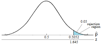
It looks like we should reject the null hypothesis because:
\[\hat{p}= 0.5172 > 0.5052\]
or equivalently since our test statistic Z = 5.49 is greater than 1.645.
Our Conclusion: We say there is sufficient evidence to conclude boys are more common than girls in the entire population.
\(p\)- value Approach Section
Next, let's state the procedure in terms of performing a proportion test using the p-value approach. The basic procedure is:
- State the null hypothesis H0 and the alternative hypothesis HA.
- Set the level of significance \(\alpha\).
- Calculate the test statistic:
\[z=\frac{\hat{p}-p_o}{\sqrt{\frac{p_0(1-p_0)}{n}}}\]
-
Calculate the p-value.
-
Make a decision. Check whether to reject the null hypothesis by comparing the p-value to \(\alpha\). If the p-value < \(\alpha\) then reject \(H_0\); otherwise do not reject \(H_0\).
Example S.6.2
Let's investigate by returning to our previous example. Again, we want to test
\(H_0: p=0.5\)
\(H_A: p>0.5\)
The test statistic
\[\begin{align} z &=\frac{\hat{p}-p_o}{\sqrt{\frac{p_0(1-p_0)}{n}}}\\
&=\frac{0.5172-0.5}{\sqrt{\frac{0.5(1-0.5)}{25468}}}\\
&= 5.49 \end{align}\]
The p-value is represented in the graph below:
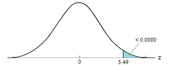
\[P = P(Z \ge 5.49) = 0.0000 \cdots \doteq 0\]
Our Conclusion: Because the p-value is smaller than the significance level \(\alpha = 0.05\), we can reject the null hypothesis. Again, we would say that there is sufficient evidence to conclude boys are more common than girls in the entire population at the \(\alpha = 0.05\) level.
As should always be the case, the two approaches, the critical value approach and the p-value approach lead to the same conclusion.