
Brinell Hardness Scores
An engineer measured the Brinell hardness of 25 pieces of ductile iron that were subcritically annealed. The resulting data were:
| Brinell Hardness of 25 Pieces of Ductile Iron | ||||||||
|---|---|---|---|---|---|---|---|---|
| 170 | 167 | 174 | 179 | 179 | 187 | 179 | 183 | 179 |
| 156 | 163 | 156 | 187 | 156 | 167 | 156 | 174 | 170 |
| 183 | 179 | 174 | 179 | 170 | 159 | 187 | ||
The engineer hypothesized that the mean Brinell hardness of all such ductile iron pieces is greater than 170. Therefore, he was interested in testing the hypotheses:
H0 : μ = 170
HA : μ > 170
The engineer entered his data into Minitab and requested that the "one-sample t-test" be conducted for the above hypotheses. He obtained the following output:
Descriptive Statistics
| N | Mean | StDev | SE Mean | 95% Lower Bound |
|---|---|---|---|---|
| 25 | 172.52 | 10.31 | 2.06 | 168.99 |
$\mu$: mean of Brinelli
Test
Null hypothesis H₀: $\mu$ = 170
Alternative hypothesis H₁: $\mu$ > 170
| T-Value | P-Value |
|---|---|
| 1.22 | 0.117 |
The output tells us that the average Brinell hardness of the n = 25 pieces of ductile iron was 172.52 with a standard deviation of 10.31. (The standard error of the mean "SE Mean", calculated by dividing the standard deviation 10.31 by the square root of n = 25, is 2.06). The test statistic t* is 1.22, and the P-value is 0.117.
If the engineer set his significance level α at 0.05 and used the critical value approach to conduct his hypothesis test, he would reject the null hypothesis if his test statistic t* were greater than 1.7109 (determined using statistical software or a t-table):
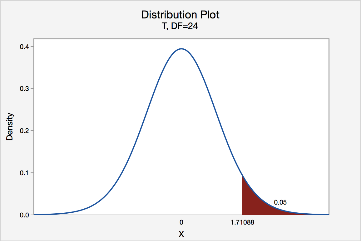
Since the engineer's test statistic, t* = 1.22, is not greater than 1.7109, the engineer fails to reject the null hypothesis. That is, the test statistic does not fall in the "critical region." There is insufficient evidence, at the \(\alpha\) = 0.05 level, to conclude that the mean Brinell hardness of all such ductile iron pieces is greater than 170.
If the engineer used the P-value approach to conduct his hypothesis test, he would determine the area under a tn - 1 = t24 curve and to the right of the test statistic t* = 1.22:
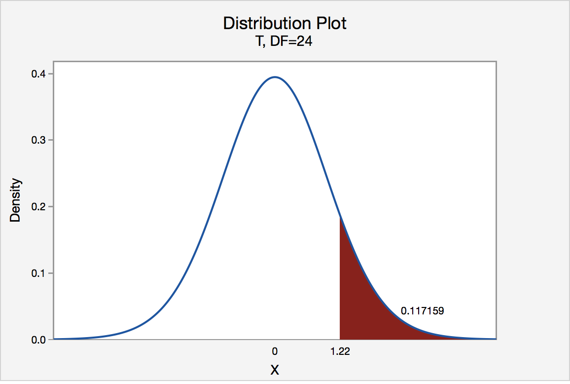
In the output above, Minitab reports that the P-value is 0.117. Since the P-value, 0.117, is greater than \(\alpha\) = 0.05, the engineer fails to reject the null hypothesis. There is insufficient evidence, at the \(\alpha\) = 0.05 level, to conclude that the mean Brinell hardness of all such ductile iron pieces is greater than 170.
Note that the engineer obtains the same scientific conclusion regardless of the approach used. This will always be the case.
Height of Sunflowers
A biologist was interested in determining whether sunflower seedlings treated with an extract from Vinca minor roots resulted in a lower average height of sunflower seedlings than the standard height of 15.7 cm. The biologist treated a random sample of n = 33 seedlings with the extract and subsequently obtained the following heights:
| Heights of 33 Sunflower Seedlings | ||||||||
|---|---|---|---|---|---|---|---|---|
| 11.5 | 11.8 | 15.7 | 16.1 | 14.1 | 10.5 | 9.3 | 15.0 | 11.1 |
| 15.2 | 19.0 | 12.8 | 12.4 | 19.2 | 13.5 | 12.2 | 13.3 | |
| 16.5 | 13.5 | 14.4 | 16.7 | 10.9 | 13.0 | 10.3 | 15.8 | |
| 15.1 | 17.1 | 13.3 | 12.4 | 8.5 | 14.3 | 12.9 | 13.5 | |
The biologist's hypotheses are:
H0 : μ = 15.7
HA : μ < 15.7
The biologist entered her data into Minitab and requested that the "one-sample t-test" be conducted for the above hypotheses. She obtained the following output:
Descriptive Statistics
| N | Mean | StDev | SE Mean | 95% Upper Bound |
|---|---|---|---|---|
| 33 | 13.664 | 2.544 | 0.443 | 14.414 |
$\mu$: mean of Height
Test
Null hypothesis H₀: $\mu$ = 15.7
Alternative hypothesis H₁: $\mu$ < 15.7
| T-Value | P-Value |
|---|---|
| -4.60 | 0.000 |
The output tells us that the average height of the n = 33 sunflower seedlings was 13.664 with a standard deviation of 2.544. (The standard error of the mean "SE Mean", calculated by dividing the standard deviation 13.664 by the square root of n = 33, is 0.443). The test statistic t* is -4.60, and the P-value, 0.000, is to three decimal places.
Minitab Note. Minitab will always report P-values to only 3 decimal places. If Minitab reports the P-value as 0.000, it really means that the P-value is 0.000....something. Throughout this course (and your future research!), when you see that Minitab reports the P-value as 0.000, you should report the P-value as being "< 0.001."
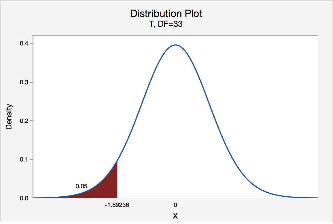
If the biologist set her significance level \(\alpha\) at 0.05 and used the critical value approach to conduct her hypothesis test, she would reject the null hypothesis if her test statistic t* were less than -1.6939 (determined using statistical software or a t-table):s-3-3
Since the biologist's test statistic, t* = -4.60, is less than -1.6939, the biologist rejects the null hypothesis. That is, the test statistic falls in the "critical region." There is sufficient evidence, at the α = 0.05 level, to conclude that the mean height of all such sunflower seedlings is less than 15.7 cm.
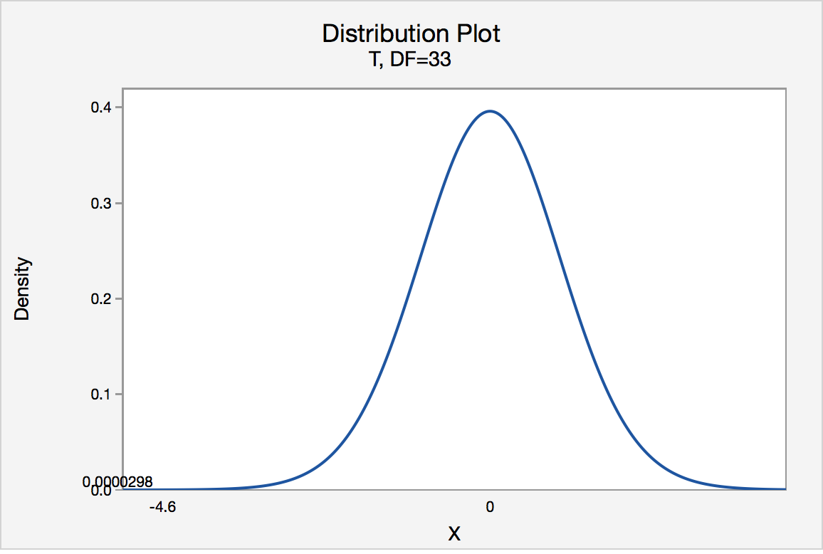
If the biologist used the P-value approach to conduct her hypothesis test, she would determine the area under a tn - 1 = t32 curve and to the left of the test statistic t* = -4.60:
In the output above, Minitab reports that the P-value is 0.000, which we take to mean < 0.001. Since the P-value is less than 0.001, it is clearly less than \(\alpha\) = 0.05, and the biologist rejects the null hypothesis. There is sufficient evidence, at the \(\alpha\) = 0.05 level, to conclude that the mean height of all such sunflower seedlings is less than 15.7 cm.
Note again that the biologist obtains the same scientific conclusion regardless of the approach used. This will always be the case.
Gum Thickness
A manufacturer claims that the thickness of the spearmint gum it produces is 7.5 one-hundredths of an inch. A quality control specialist regularly checks this claim. On one production run, he took a random sample of n = 10 pieces of gum and measured their thickness. He obtained:
| Thicknesses of 10 Pieces of Gum | ||||
|---|---|---|---|---|
| 7.65 | 7.60 | 7.65 | 7.70 | 7.55 |
| 7.55 | 7.40 | 7.40 | 7.50 | 7.50 |
The quality control specialist's hypotheses are:
H0 : μ = 7.5
HA : μ ≠ 7.5
The quality control specialist entered his data into Minitab and requested that the "one-sample t-test" be conducted for the above hypotheses. He obtained the following output:
Descriptive Statistics
| N | Mean | StDev | SE Mean | 95% CI for $\mu$ |
|---|---|---|---|---|
| 10 | 7.550 | 0.1027 | 0.0325 | (7.4765, 7.6235) |
$\mu$: mean of Thickness
Test
Null hypothesis H₀: $\mu$ = 7.5
Alternative hypothesis H₁: $\mu \ne$ 7.5
| T-Value | P-Value |
|---|---|
| 1.54 | 0.158 |
The output tells us that the average thickness of the n = 10 pieces of gums was 7.55 one-hundredths of an inch with a standard deviation of 0.1027. (The standard error of the mean "SE Mean", calculated by dividing the standard deviation 0.1027 by the square root of n = 10, is 0.0325). The test statistic t* is 1.54, and the P-value is 0.158.
If the quality control specialist sets his significance level \(\alpha\) at 0.05 and used the critical value approach to conduct his hypothesis test, he would reject the null hypothesis if his test statistic t* were less than -2.2616 or greater than 2.2616 (determined using statistical software or a t-table):
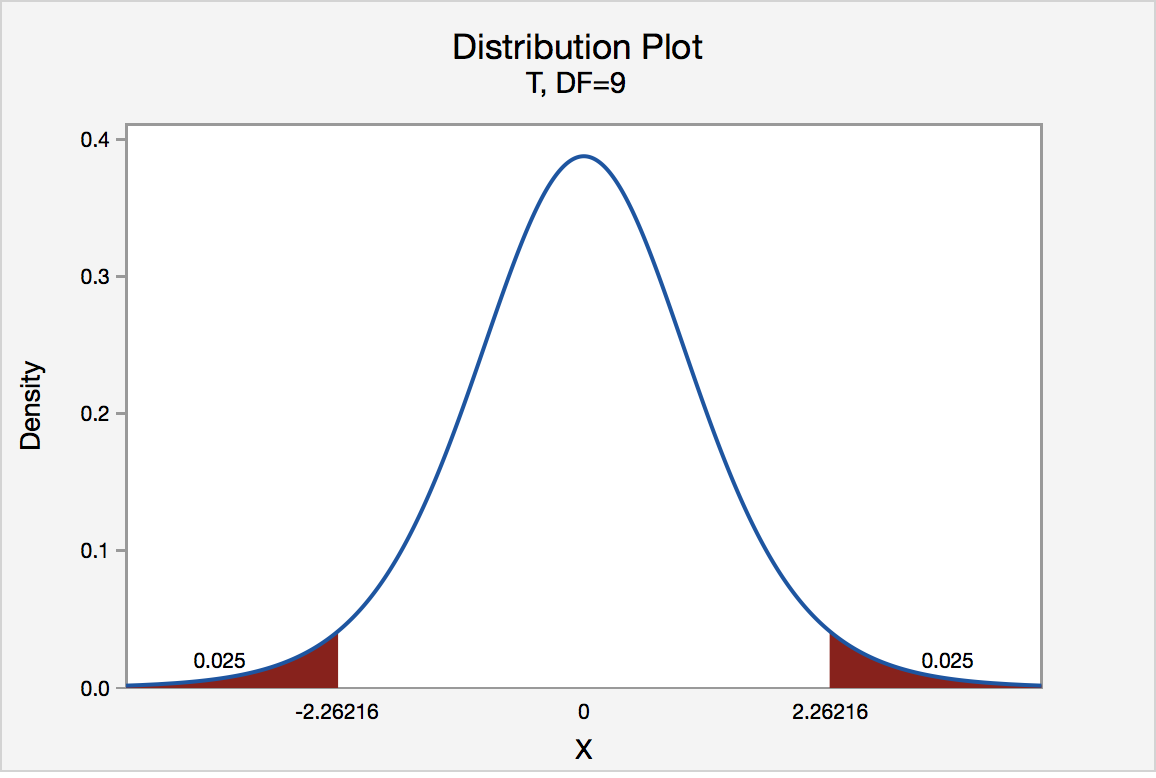
Since the quality control specialist's test statistic, t* = 1.54, is not less than -2.2616 nor greater than 2.2616, the quality control specialist fails to reject the null hypothesis. That is, the test statistic does not fall in the "critical region." There is insufficient evidence, at the \(\alpha\) = 0.05 level, to conclude that the mean thickness of all of the manufacturer's spearmint gum differs from 7.5 one-hundredths of an inch.
If the quality control specialist used the P-value approach to conduct his hypothesis test, he would determine the area under a tn - 1 = t9 curve, to the right of 1.54 and to the left of -1.54:
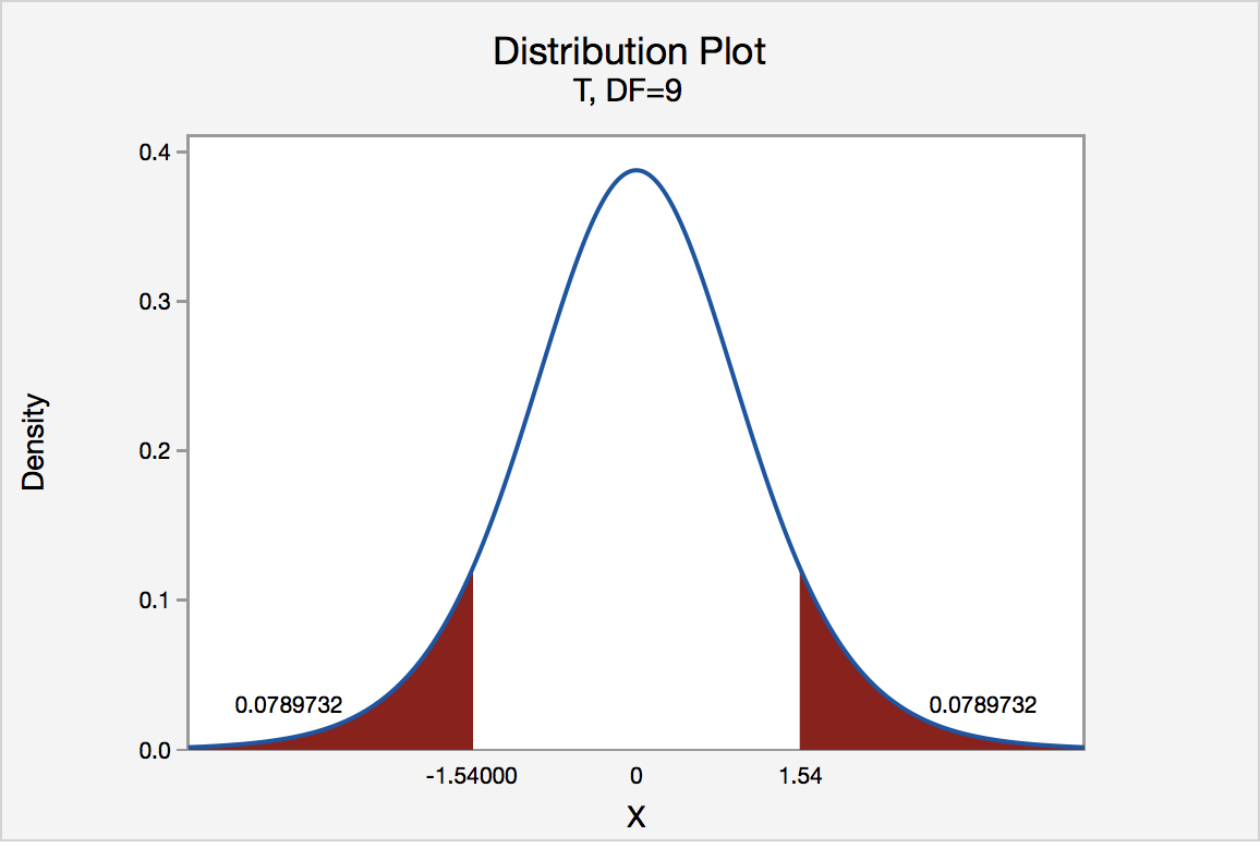
In the output above, Minitab reports that the P-value is 0.158. Since the P-value, 0.158, is greater than \(\alpha\) = 0.05, the quality control specialist fails to reject the null hypothesis. There is insufficient evidence, at the \(\alpha\) = 0.05 level, to conclude that the mean thickness of all pieces of spearmint gum differs from 7.5 one-hundredths of an inch.
Note that the quality control specialist obtains the same scientific conclusion regardless of the approach used. This will always be the case.
In closing
In our review of hypothesis tests, we have focused on just one particular hypothesis test, namely that concerning the population mean \(\mu\). The important thing to recognize is that the topics discussed here — the general idea of hypothesis tests, errors in hypothesis testing, the critical value approach, and the P-value approach — generally extend to all of the hypothesis tests you will encounter.