
Why is Power Analysis Important? Section
Consider a research experiment where the p-value computed from the data was 0.12. As a result, one would fail to reject the null hypothesis because this p-value is larger than \(\alpha\) = 0.05. However, there still exist two possible cases for which we failed to reject the null hypothesis:
- the null hypothesis is a reasonable conclusion,
- the sample size is not large enough to either accept or reject the null hypothesis, i.e., additional samples might provide additional evidence.
Power analysis is the procedure that researchers can use to determine if the test contains enough power to make a reasonable conclusion. From another perspective power analysis can also be used to calculate the number of samples required to achieve a specified level of power.
Example S.5.1
Let's take a look at an example that illustrates how to compute the power of the test.
Example
Let X denote the height of randomly selected Penn State students. Assume that X is normally distributed with unknown mean \(\mu\) and a standard deviation of 9. Take a random sample of n = 25 students, so that, after setting the probability of committing a Type I error at \(\alpha = 0.05\), we can test the null hypothesis \(H_0: \mu = 170\) against the alternative hypothesis that \(H_A: \mu > 170\).
What is the power of the hypothesis test if the true population mean were \(\mu = 175\)?
\[\begin{align}z&=\frac{\bar{x}-\mu}{\sigma / \sqrt{n}} \\
\bar{x}&= \mu + z \left(\frac{\sigma}{\sqrt{n}}\right) \\
\bar{x}&=170+1.645\left(\frac{9}{\sqrt{25}}\right) \\
&=172.961\\
\end{align}\]
So we should reject the null hypothesis when the observed sample mean is 172.961 or greater:
We get
\[\begin{align}\text{Power}&=P(\bar{x} \ge 172.961 \text{ when } \mu =175)\\
&=P\left(z \ge \frac{172.961-175}{9/\sqrt{25}} \right)\\
&=P(z \ge -1.133)\\
&= 0.8713\\
\end{align}\]
and illustrated below:
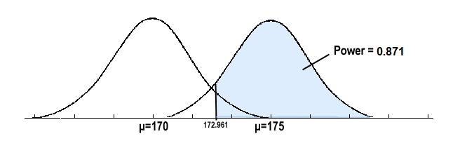
In summary, we have determined that we have an 87.13% chance of rejecting the null hypothesis \(H_0: \mu = 170\) in favor of the alternative hypothesis \(H_A: \mu > 170\) if the true unknown population mean is, in reality, \(\mu = 175\).
Calculating Sample Size Section
If the sample size is fixed, then decreasing Type I error \(\alpha\) will increase Type II error \(\beta\). If one wants both to decrease, then one has to increase the sample size.
To calculate the smallest sample size needed for specified \(\alpha\), \(\beta\), \(\mu_a\), then (\(\mu_a\) is the likely value of \(\mu\) at which you want to evaluate the power.
- Sample Size for One-Tailed Test
- \(n = \dfrac{\sigma^2(Z_{\alpha}+Z_{\beta})^2}{(\mu_0−\mu_a)^2}\)
- Sample Size for Two-Tailed Test
- \(n = \dfrac{\sigma^2(Z_{\alpha/2}+Z_{\beta})^2}{(\mu_0−\mu_a)^2}\)
Let's investigate by returning to our previous example.
Example S.5.2
Let X denote the height of randomly selected Penn State students. Assume that X is normally distributed with unknown mean \(\mu\) and standard deviation 9. We are interested in testing at \(\alpha = 0.05\) level , the null hypothesis \(H_0: \mu = 170\) against the alternative hypothesis that \(H_A: \mu > 170\).
Find the sample size n that is necessary to achieve 0.90 power at the alternative μ = 175.
\[\begin{align}n&= \dfrac{\sigma^2(Z_{\alpha}+Z_{\beta})^2}{(\mu_0−\mu_a)^2}\\ &=\dfrac{9^2 (1.645 + 1.28)^2}{(170-175)^2}\\ &=27.72\\ n&=28\\ \end{align}\]
In summary, you should see how power analysis is very important so that we are able to make the correct decision when the data indicate that one cannot reject the null hypothesis. You should also see how power analysis can also be used to calculate the minimum sample size required to detect a difference that meets the needs of your research.