The critical value approach involves determining "likely" or "unlikely" by determining whether or not the observed test statistic is more extreme than would be expected if the null hypothesis were true. That is, it entails comparing the observed test statistic to some cutoff value, called the "critical value." If the test statistic is more extreme than the critical value, then the null hypothesis is rejected in favor of the alternative hypothesis. If the test statistic is not as extreme as the critical value, then the null hypothesis is not rejected.
Specifically, the four steps involved in using the critical value approach to conducting any hypothesis test are:
- Specify the null and alternative hypotheses.
- Using the sample data and assuming the null hypothesis is true, calculate the value of the test statistic. To conduct the hypothesis test for the population mean μ, we use the t-statistic \(t^*=\frac{\bar{x}-\mu}{s/\sqrt{n}}\) which follows a t-distribution with n - 1 degrees of freedom.
- Determine the critical value by finding the value of the known distribution of the test statistic such that the probability of making a Type I error — which is denoted \(\alpha\) (greek letter "alpha") and is called the "significance level of the test" — is small (typically 0.01, 0.05, or 0.10).
- Compare the test statistic to the critical value. If the test statistic is more extreme in the direction of the alternative than the critical value, reject the null hypothesis in favor of the alternative hypothesis. If the test statistic is less extreme than the critical value, do not reject the null hypothesis.
Example S.3.1.1
Mean GPA Section
In our example concerning the mean grade point average, suppose we take a random sample of n = 15 students majoring in mathematics. Since n = 15, our test statistic t* has n - 1 = 14 degrees of freedom. Also, suppose we set our significance level α at 0.05 so that we have only a 5% chance of making a Type I error.
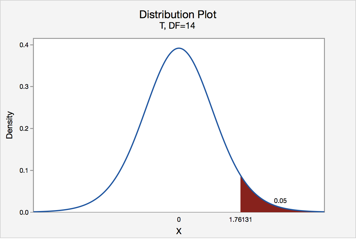
Right-Tailed
The critical value for conducting the right-tailed test H0 : μ = 3 versus HA : μ > 3 is the t-value, denoted t\(\alpha\), n - 1, such that the probability to the right of it is \(\alpha\). It can be shown using either statistical software or a t-table that the critical value t 0.05,14 is 1.7613. That is, we would reject the null hypothesis H0 : μ = 3 in favor of the alternative hypothesis HA : μ > 3 if the test statistic t* is greater than 1.7613. Visually, the rejection region is shaded red in the graph.
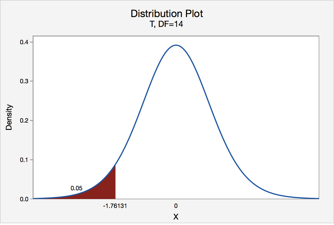
Left-Tailed
The critical value for conducting the left-tailed test H0 : μ = 3 versus HA : μ < 3 is the t-value, denoted -t(\(\alpha\), n - 1), such that the probability to the left of it is \(\alpha\). It can be shown using either statistical software or a t-table that the critical value -t0.05,14 is -1.7613. That is, we would reject the null hypothesis H0 : μ = 3 in favor of the alternative hypothesis HA : μ < 3 if the test statistic t* is less than -1.7613. Visually, the rejection region is shaded red in the graph.
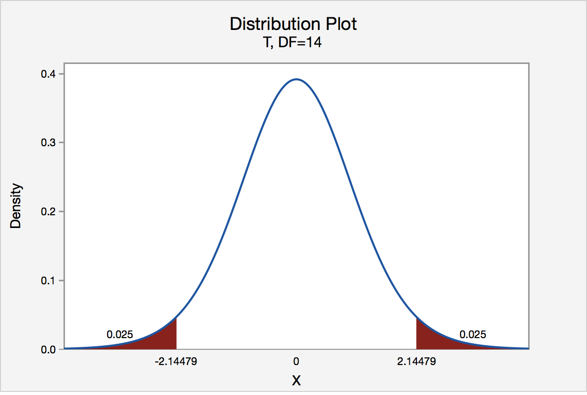
Two-Tailed
There are two critical values for the two-tailed test H0 : μ = 3 versus HA : μ ≠ 3 — one for the left-tail denoted -t(\(\alpha\)/2, n - 1) and one for the right-tail denoted t(\(\alpha\)/2, n - 1). The value -t(\(\alpha\)/2, n - 1) is the t-value such that the probability to the left of it is \(\alpha\)/2, and the value t(\(\alpha\)/2, n - 1) is the t-value such that the probability to the right of it is \(\alpha\)/2. It can be shown using either statistical software or a t-table that the critical value -t0.025,14 is -2.1448 and the critical value t0.025,14 is 2.1448. That is, we would reject the null hypothesis H0 : μ = 3 in favor of the alternative hypothesis HA : μ ≠ 3 if the test statistic t* is less than -2.1448 or greater than 2.1448. Visually, the rejection region is shaded red in the graph.