Example 11-3: Place Rated (after Standardization) Section
The SAS program implements the principal component procedures with standardized data:
download the SAS Program here: places1.sas
Note: In the upper right-hand corner of the code block you will have the option of copying ( ) the code to your clipboard or downloading ( ) the file to your computer.
options ls=78;
title "PCA - Correlation Matrix - Places Rated";

 /* After reading in the places data, the (base 10) log transformations are taken.
  * This is an optional step and not required for the pca analysis.
  */

data places;
  infile "D:\Statistics\STAT 505\data\places.csv" firstobs=2 delimiter=',';
  input climate housing health crime trans educate arts recreate econ id;
  climate=log10(climate);
  housing=log10(housing);
  health=log10(health);
  crime=log10(crime);
  trans=log10(trans);
  educate=log10(educate);
  arts=log10(arts);
  recreate=log10(recreate);
  econ=log10(econ);
  run;

 /* The princomp procedure performs pca on the correlation matrix.
  * The out=a option saves results to a data set named 'a'.
  */

proc princomp data=places out=a;
  var climate housing health crime trans educate arts recreate econ;
  run;

 /* The corr procedure is used to calculate pairwise correlations
  * between the first 3 principal components and the original variables.
  */

proc corr data=a;
  var prin1 prin2 prin3 climate housing health crime trans educate arts
      recreate econ;
  run;

proc gplot data=a;
  axis1 length=5 in;
  axis2 length=5 in;
  plot prin2*prin1 / vaxis=axis1 haxis=axis2;
  run;
The output begins with descriptive information including the means and standard deviations for the individual variables presented.
This is followed by the Correlation Matrix for the data. For example, the correlation between the housing and climate data was only 0.273. There are no hypotheses presented that these correlations are equal to zero. We will use this correlation matrix instead to obtain our eigenvalues and eigenvectors.
Principal components analysis (correlation matrix)
To perform principal components analysis on the correlation matrix
- Open the ‘places’ data set in a new worksheet.
- Transform variables. This step is optional but used in the steps below.
- Calc > Calculator
- Highlight and select ‘climate’ to move it to the Store result window.
- In the Expression window, enter LOGTEN( 'climate') to apply the (base 10) log transformation to the climate variable.
- Choose OK. The transformed values replace the originals in the worksheet under ‘climate’.
- Repeat sub-steps 1) through 4) above for all variables housing through econ.
- Stat > Multivariate > Principal Components
- Highlight and select climate through econ to move all 9 variables to the Variables window.
- Choose 9 for number of components.
- Check Correlation for Type of Matrix.
- Under Storage, for the Coefficients and Eigenvalues, enter c11 and c12 (or any two unused columns in the worksheet).
- Choose OK and OK again. The results are displayed in the results area and stored in worksheet columns as well.
Analysis
We need to focus on the eigenvalues of the correlation matrix that correspond to each of the principal components. In this case, the total variation of the standardized variables is equal to p, the number of variables. After standardization, each variable has a variance equal to one, and the total variation is the sum of these variations, in this case, the total variation will be 9.
The eigenvalues of the correlation matrix are given in the second column in the table below. The proportion of variation explained by each of the principal components as well as the cumulative proportion of the variation explained are also provided.
Step 1
Examine the eigenvalues to determine how many principal components to consider:
| Component | Eigenvalue | Proportion | Cumulative |
|---|---|---|---|
| 1 | 3.2978 | 0.3664 | 0.3664 |
| 2 | 1.2136 | 0.1348 | 0.5013 |
| 3 | 1.1055 | 0.1228 | 0.6241 |
| 4 | 0.9073 | 0.1008 | 0.7249 |
| 5 | 0.8606 | 0.0956 | 0.8205 |
| 6 | 0.5622 | 0.0625 | 0.8830 |
| 7 | 0.4838 | 0.0538 | 0.9368 |
| 8 | 0.3181 | 0.0353 | 0.9721 |
| 9 | 0.2511 | 0.0279 | 1.0000 |
The first principal component explains about 37% of the variation. Furthermore, the first four principal components explain 72%, while the first five principal components explain 82% of the variation. Compare these proportions with those obtained using non-standardized variables. This analysis is going to require a larger number of components to explain the same amount of variation as the original analysis using the variance-covariance matrix. This is not unusual.
In most cases, the required cut-off is pre-specified; i.e. how much of the variation to be explained is pre-determined. For instance, I might state that I would be satisfied if I could explain 70% of the variation. If we do this, then we would select the components necessary until you get up to 70% of the variation. This would be one approach. This type of judgment is arbitrary and hard to make if you are not experienced with these types of analysis. The goal - to some extent - also depends on the type of problem at hand.
Another approach would be to plot the differences between the ordered values and look for a break or a sharp drop. The only sharp drop that is noticeable in this case is after the first component. One might based on this, select only one component. However, one component is probably too few, particularly because we have only explained 37% of the variation. Consider the scree plot based on the standardized variables.
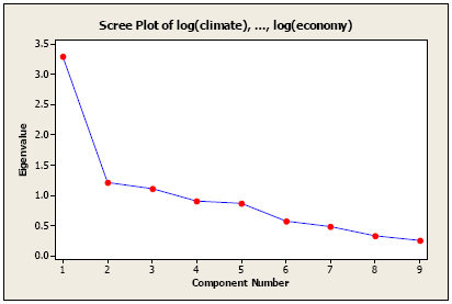
The scree plot for standardized variables (correlation matrix)
Step 2
Next, we can compute the principal component scores using the eigenvectors. This is a formula for the first principal component:
\(\begin{array} \hat{Y}_1 & = & 0.158 \times Z_{\text{climate}} + 0.384 \times Z_{\text{housing}} + 0.410 \times Z_{\text{health}}\\ & & + 0.259 \times Z_{\text{crime}} + 0.375 \times Z_{\text{transportation}} + 0.274 \times Z_{\text{education}} \\ && 0.474 \times Z_{\text{arts}} + 0.353 \times Z_{\text{recreation}} + 0.164 \times Z_{\text{economy}}\end{array}\)
And remember, this is now a function of the standardized data, not of the raw data.
The magnitudes of the coefficients give the contributions of each variable to that component. Because the data have been standardized, they do not depend on the variances of the corresponding variables.
Step 3
Let's look at the coefficients for the principal components. In this case, because the data are standardized, the relative magnitude of each coefficient can be directly assessed within a column. Each column here corresponds with a column in the output of the program labeled Eigenvectors.
| Principal Component | |||||
|---|---|---|---|---|---|
| Variable | 1 | 2 | 3 | 4 | 5 |
| Climate | 0.158 | 0.069 | 0.800 | 0.377 | 0.041 |
| Housing | 0.384 | 0.139 | 0.080 | 0.197 | -0.580 |
| Health | 0.410 | -0.372 | -0.019 | 0.113 | 0.030 |
| Crime | 0.259 | 0.474 | 0.128 | -0.042 | 0.692 |
| Transportation | 0.375 | -0.141 | -0.141 | -0.430 | 0.191 |
| Education | 0.274 | -0.452 | -0.241 | 0.457 | 0.224 |
| Arts | 0.474 | -0.104 | 0.011 | -0.147 | 0.012 |
| Recreation | 0.353 | 0.292 | 0.042 | -0.404 | -0.306 |
| Economy | 0.164 | 0.540 | -0.507 | 0.476 | -0.037 |
Interpretation of the principal components is based on which variables are most strongly correlated with each component. In other words, we need to decide which numbers are large within each column. In the first column, we see that Health and Arts are large. This is very arbitrary. Other variables might have also been included as part of this first principal component.
Component Summaries Section
- First Principal Component Analysis - PCA1
The first principal component is a measure of the quality of Health and the Arts, and to some extent Housing, Transportation, and Recreation. This component is associated with high ratings on all of these variables, especially Health, and Arts. They are all positively related to PCA1 because they all have positive signs.
- Second Principal Component Analysis - PCA2
The second principal component is a measure of the severity of the crime, the quality of the economy, and the lack of quality education. PCA2 is associated with high ratings of Crime and Economy and low ratings of Education. Here we can see that PCA2 distinguishes cities with high levels of crime and good economies from cities with poor educational systems.
- Third Principal Component Analysis - PCA3
The third principal component is a measure of the quality of the climate and the poorness of the economy. PCA3 is associated with high Climate ratings and low Economy ratings. The inclusion of economy within this component will add a bit of redundancy to our results. This component is primarily a measure of climate and to a lesser extent the economy.
- Fourth Principal Component Analysis - PCA4
The fourth principal component is a measure of the quality of education and the economy and the poorness of the transportation network and recreational opportunities. PCA4 is associated with high Education and Economy ratings and low Transportation and Recreation ratings.
- Fifth Principal Component Analysis - PCA5
The fifth principal component is a measure of the severity of the crime and the quality of housing. PCA5 is associated with high Crime ratings and low housing ratings.