Recall the Multivariate Normal Density function below:
\(\phi(\textbf{x}) = \left(\frac{1}{2\pi}\right)^{p/2}|\Sigma|^{-1/2}\exp\{-\frac{1}{2}(\textbf{x}-\mathbf{\mu})'\Sigma^{-1}(\textbf{x}-\mathbf{\mu})\}\)
You will note that this density function, \(\phi(\textbf{x})\), only depends on x through the squared Mahalanobis distance:
\((\textbf{x}-\mathbf{\mu})'\Sigma^{-1}(\textbf{x}-\mathbf{\mu})\)
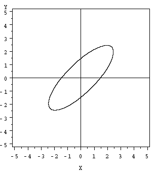
This is the equation for a hyper-ellipse centered at \(\mu\).
For a bivariate normal, where p = 2 variables, we have an ellipse as shown in the plot below:

Useful facts about the Exponent Component: \( (\textbf{x}-\mathbf{\mu})'\Sigma^{-1}(\textbf{x}-\mathbf{\mu})\)
- All values of x such that \( (\textbf{x}-\mathbf{\mu})'\Sigma^{-1}(\textbf{x}-\mathbf{\mu})=c\) for any specified constant value c have the same value of the density \(f(x)\) and thus have an equal likelihood.
- As the value of \((\textbf{x}-\mathbf{\mu})'\Sigma^{-1}(\textbf{x}-\mathbf{\mu})\) increases, the value of the density function decreases. The value of \((\textbf{x}-\mathbf{\mu})'\Sigma^{-1}(\textbf{x}-\mathbf{\mu})\) increases as the distance between x and \(\mu\) increases.
- The variable \(d^2=(\textbf{x}-\mathbf{\mu})'\Sigma^{-1}(\textbf{x}-\mathbf{\mu})\) has a chi-square distribution with p degrees of freedom.
- The value of d 2 for a specific observation \(\textbf{x}_j\) is called a squared Mahalanobis distance.
- Squared Mahalanobis Distance
- \(d^2_j = (\textbf{x}_j-\mathbf{\bar{x}})'\Sigma^{-1}(\textbf{x}_j-\mathbf{\bar{x}})\)
If we define a specific hyper-ellipse by taking the squared Mahalanobis distance equal to a critical value of the chi-square distribution with p degrees of freedom and evaluate this at \(α\), then the probability that the random value X will fall inside the ellipse is going to be equal to \(1 - α\).
\(\text{Pr}\{(\textbf{x}-\mathbf{\mu})'\Sigma^{-1}(\textbf{x}-\mathbf{\mu}) \le \chi^2_{p,\alpha}\}=1-\alpha\)
This particular ellipse is called the \((1 - α) \times 100%\) prediction ellipse for a multivariate normal random vector with mean vector \(\mu\) and variance-covariance matrix \(Σ\).
Using Technology Section
Calculating Mahalanobis Distance With SAS
SAS does not provide Mahalanobis distance directly, but we can compute them using principal components. The steps are:
- Determine the principal components for the correlation matrix of the x-variables.
- Standardize the principal component scores so that each principal component has a standard deviation = 1. For each component, this is done by dividing the scores by the square root of the eigenvalue. In SAS, use the STD option as part of the PROC PRINCOMP command to automate this standard deviation.
- For each observation, calculate \(d^{2}\) = sum of squared standardized principal components scores. This will equal the squared Mahalanobis distance.
Example - Calculating and Printing Mahalonobis Distances in SAS
Suppose we have four x-variables, called \(x_1 , x_2 , x_3 , x_4\), and they have already been read into SAS. The following SAS code (Download below) will determine standardized principal components and calculate Mahalanobis distances (the printout will include observation numbers). Within the DATA step, the “uss(of prin1-prin4)” function calculates the uncorrected sum of squares for the variables prin1-prin4. This value will be computed for each observation in the “pcout” data set. The result of the DATA step will be a SAS data set named “mahal” that will include the original variables, the standardized principal component scores (named prin1-prin4), and the Mahalanobis distance (named dist2).
Data file: boardstiffness.csv
Note: In the upper right-hand corner of the code block you will have the option of copying ( ) the code to your clipboard or downloading ( ) the file to your computer.
data boards; /*This defines the name of the data set with the name 'boards'.*/
infile "D:\stat505data\boardstiffness.csv" firstobs=2 delimiter=',';   /*This is the path where the contents of the data set are read from.*/
input x1 x2 x3 x4;   /*This is where we provide names for the variables in order of the columns in the data set. If any were categorical (not the case here), we would need to put a '$' character after its name.*/
run;

proc princomp std out=pcresult;   /*The princomp procedure is primarily used for principal components analysis, which we will see later in this course, but it also provides the Mahalanobis distances we need for producing the QQ plot. The 'out' option specifies the name of a data set used to store results from this procedure.*/
var x1 x2 x3 x4;   /*This specifies that the four variables specified will be used in the princomp calculations.*/
run;

data mahal;
set pcresult;   /*This makes the variables in the previously defined data set 'pcresult' available for this new data set 'mahal'.*/
dist2=uss(of prin1-prin4);   /*This calculates the squared Mahalanobis distances from the output generated from the princomp procedure above.*/
run;

proc print data=mahal;   /*This prints the specified variable(s) from the data set 'mahal'.*/
var dist2;   /*Only the 'dist2' variable will be printed in this case.*/
run;
To calculate the Mahalanobis distances in Minitab:
- Open the ‘boardstiffness’ data set in a new worksheet. Note that this particular data set already has the squared distances as the last column, which will not be used in the calculations here.
- Stat > Multivariate > Principal Components
- Highlight and select the first four variables (‘C1’ through ‘C4’) to move them into the ‘Variables’ window
- Select ‘Storage’ and enter a new column name, such as ‘Mahal’ in the ‘Distances’ window. This is where the calculated distance values will be stored.
- Select ‘OK’ and ‘OK’ again. The Mahalanobis distances should appear in the worksheet under the column name provided in step 4.