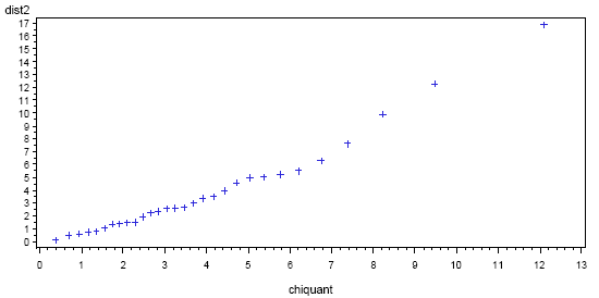
Q-Q Plot for Evaluating Multivariate Normality and Outliers Section
The variable \(d^2 = (\textbf{x}-\mathbf{\mu})'\Sigma^{-1}(\textbf{x}-\mathbf{\mu})\) has a chi-square distribution with p degrees of freedom, and for “large” samples the observed Mahalanobis distances have an approximate chi-square distribution. This result can be used to evaluate (subjectively) whether a data point may be an outlier and whether observed data may have a multivariate normal distribution.
A Q-Q plot can be used to picture the Mahalanobis distances for the sample. The basic idea is the same as for a normal probability plot. For multivariate data, we plot the ordered Mahalanobis distances versus estimated quantiles (percentiles) for a sample of size n from a chi-squared distribution with p degrees of freedom. This should resemble a straight line for data from a multivariate normal distribution. Outliers will show up as points on the upper right side of the plot for which the Mahalanobis distance is notably greater than the chi-square quantile value.
Determining the Quantiles
- The \(i^{th}\) estimated quantile is determined as the chi-square value (with df = p) for which the cumulative probability is (i - 0.5) / n.
- To determine the full set of estimated chi-square quantiles, this is done for the value of i from 1 to n.
Example 4-2: Q-Q Plot for Board Stiffness Data Section
This example reproduces Example 4.14 in the text (page 187). For each n = 30 boards, there are p = 4 measurements of board stiffness. Each measurement was done using a different method.
A SAS plot of the Mahalanobis distances is given below. The distances are on the vertical axis and the chi-square quantiles are on the horizontal axis. On the right side of the plot, we see an upward bending. This indicates possible outliers (and a possible violation of multivariate normality). In particular, the final point has \(d^{2}≈ 16\) whereas the quantile value on the horizontal is about 12.5. The next-to-last point in the plot might also be an outlier. A printout of the distances, before they were ordered for the plot, shows that the two possible outliers are boards 16 and 9, respectively.

The SAS code used to produce the above graph is as follows:
The data step reads the dataset.
Note: In the upper right-hand corner of the code block you will have the option of copying ( ) the code to your clipboard or downloading ( ) the file to your computer.
data boards;   /*This defines the name of the data set with the name 'boards'.*/
infile "D:\stat505data\boardstiffness.csv" firstobs=2 delimiter=',';   /*This is the path where the contents of the data set are read from.*/
input x1 x2 x3 x4;   /*This is where we provide names for the variables in order of the columns in the data set. If any were categorical (not the case here), we would need to put a '$' character after its name.*/
run;

proc princomp std out=pcresult;   /*The princomp procedure is primarily used for principal components analysis, which we will see later in this course, but it also provides the Mahalanobis distances we need for producing the QQ plot. The 'out' option specifies the name of a data set used to store results from this procedure.*/
var x1 x2 x3 x4;   /*This specifies that the four variables specified will be used in the princomp calculations.*/
run;

data mahal;
set pcresult;   /*This makes the variables in the previously defined data set 'pcresult' available for this new data set 'mahal'.*/
dist2=uss(of prin1-prin4);   /*This calculates the squared Mahalanobis distances from the output generated from the princomp procedure above.*/
run;

proc print;   /*This prints the specified variable(s) from the data set 'mahal'.*/
var dist2;   /*Only the 'dist2' variable will be printed in this case.*/
run;

proc sort;   /*This sorts the data set 'mahal' by the variable 'dist2'. We need to do this before constructing the QQ plot in order to match up the squared distances against the correct chi-square quantiles.*/
by dist2;
run;

data plotdata;   /*This defines the data set 'plotdata'.*/
set mahal;   /*This makes use of the previously defined data set 'mahal'.*/
prb=(_n_ -.5)/30;   /*This calculates the probabilities to be used in the chi-square quantiles. The _n_ object provides the numbers 1 to 30 (the sample size), and by dividing by the sample size, we effectively divide the range 0 to 1 into 30 points. However, we subtract by 0.5 in order to avoid the limit of 1, since the chi-square quantile at 1 is infinite.*/
chiquant=cinv(prb,4);
run;

proc gplot;   /*This produces the QQ plot between the squared distances and the chi-square quantiles computed above.*/
plot dist2*chiquant;
run;
How to Produce a QQ plot for the Board Stiffness Dataset using Minitab
To construct a QQ plot in Minitab
- Open the ‘boardstiffness’ data set in a new worksheet, and calculate the Mahalanobis distances. The steps below assume these distances are stored in the worksheet column ‘Mahal’.
- Calc > Calculator
- In ‘Store result in variable’, enter the name of a new column, such as C7.
- In the expression window, enter Mahal**2 to square the values of the Mahalanobis distances.
- Select ‘OK’. The squared Mahalanobis distances should appear in the worksheet under C7.
- Rename the new column to ‘Mahal2’ for convenience.
- Graph > Probability Plot > Simple
- Highlight and select ‘Mahal2’ to move it to the ‘Graph variables’ window.
- Choose the ‘Distribution’ button and specify.
- Distribution > Gamma (the chi-square is a special case of the gamma)
- Shape > 2 for the number of variables divided by 2; in general, this will depend on the number of variables considered for the plot.
- Scale > 2
- Select ‘OK’.
- Choose the ‘Scale’ button and check ‘Transpose Y and X’.
- Select ‘OK’. The QQ plot should appear in the results area.