Example: Woodyard Hammock Data Section
SAS uses the Euclidian distance metric and agglomerative clustering, while Minitab can use Manhattan, Pearson, Squared Euclidean, and Squared Pearson distances as well. Both SAS and Minitab use only agglomerative clustering.
Use the datafile wood.csv.
Cluster analysis is carried out in SAS using a cluster analysis procedure that is abbreviated as a cluster. We will look at how this is carried out in the SAS program below.
options ls=78;
title 'Cluster Analysis - Woodyard Hammock - Complete Linkage';

data wood;
  infile 'D:\Statistics\STAT 505\data\wood.csv' firstobs=2 delimiter=',';
  input x y acerub carcar carcor cargla cercan corflo faggra frapen
        ileopa liqsty lirtul maggra magvir morrub nyssyl osmame ostvir
        oxyarb pingla pintae pruser quealb quehem quenig quemic queshu quevir
        symtin ulmala araspi cyrrac;
  ident=_n_;
  drop acerub carcor cargla cercan frapen lirtul magvir morrub osmame pintae
       pruser quealb quehem queshu quevir ulmala araspi cyrrac;
  run;

proc sort data=wood;
  by ident;
  run;

proc cluster data=wood method=complete outtree=clust1;
  var carcar corflo faggra ileopa liqsty maggra nyssyl ostvir oxyarb
      pingla quenig quemic symtin;
  id ident;
  run;

proc tree data=clust1 horizontal nclusters=6 out=clust2;
  id ident;
  run;

proc sort data=clust2;
  by ident;
  run;

proc print data=clust2;
  run;

data combine;
  merge wood clust2;
  by ident;
  run;

proc glm data=combine;
  class cluster;
  model carcar corflo faggra ileopa liqsty maggra nyssyl ostvir oxyarb
        pingla quenig quemic symtin = cluster;
  means cluster;
  run;
Download the SAS Program here: wood1.sas
Note: In the upper right-hand corner of the code block you will have the option of copying ( ) the code to your clipboard or downloading ( ) the file to your computer.
options ls=78;
title 'Cluster Analysis - Woodyard Hammock - Complete Linkage';

 /* After reading in the data, an ident variable is created as the
  * row number for each observation. This is neeed for the clustering algorithm.
  * The drop statement removes several variables not used for this analysis.
  */

data wood;
  infile 'D:\Statistics\STAT 505\data\wood.csv' firstobs=2 delimiter=',';
  input x y acerub carcar carcor cargla cercan corflo faggra frapen
        ileopa liqsty lirtul maggra magvir morrub nyssyl osmame ostvir
        oxyarb pingla pintae pruser quealb quehem quenig quemic queshu quevir
        symtin ulmala araspi cyrrac;
  ident=_n_;
  drop acerub carcor cargla cercan frapen lirtul magvir morrub osmame pintae
       pruser quealb quehem queshu quevir ulmala araspi cyrrac;
  run;

 /* The observations are sorted by their ident value.
  */

proc sort data=wood;
  by ident;
  run;

 /* The cluster procedure is for hierarchical clustering.
  * The method option specifies the cluster distance formula to use.
  * The outtree option saves the results.
  */

proc cluster data=wood method=complete outtree=clust1;
  var carcar corflo faggra ileopa liqsty maggra nyssyl ostvir oxyarb
      pingla quenig quemic symtin;
  id ident;
  run;

 /* The tree procedure generates a dendrogram of the heirarchical
  * clustering results and saves cluster label assignments if the
  * nclusters option is also specified.
  */

proc tree data=clust1 horizontal nclusters=6 out=clust2;
  id ident;
  run;

 /* The data are sorted by their ident value.
  */

proc sort data=clust2;
  by ident;
  run;

 /* The results from clust2 are printed.
  */

proc print data=clust2;
  run;

 /* This step combines the original wood data set with
  * the results of clust2, which allows the ANOVA statistics
  * to be calculated in the following glm procedure.
  */

data combine;
  merge wood clust2;
  by ident;
  run;

 /* The glm procedure views the cluster labels as ANOVA groups and
  * reports several statistics to assess variation between clusters
  * relative to variation within clusters.
  * The mean for each cluster is also reported.
  */

proc glm data=combine;
  class cluster;
  model carcar corflo faggra ileopa liqsty maggra nyssyl ostvir oxyarb
        pingla quenig quemic symtin = cluster;
  means cluster;
  run;
Performing a cluster analysis
To perform cluster analysis:
- Open the ‘wood’ data set in a new worksheet.
- Stat > Multivariate > Cluster Observations
- Highlight and select the variables to use in the clustering. For this example, the following variables are selected (13 total): carcar corflo faggra ileopa liqsty maggra nyssyl ostvir oxyarb pingla quenig quemic symtin
- Choose Complete as the Linkage and Euclidean as the Distance.
- Choose Show dendrogram, and under Customize, choose Distance for Y Axis.
- Choose OK, and OK again. The results, along with the dendrogram, are shown in the session window.
Dendrograms (Tree Diagrams) Section
The results of cluster analysis are best summarized using a dendrogram. In a dendrogram, distance is plotted on one axis, while the sample units are given on the remaining axis. The tree shows how the sample units are combined into clusters, the height of each branching point corresponding to the distance at which two clusters are joined.
In looking at the cluster history section of the SAS (or Minitab) output, we see that the Euclidean distance between sites 33 and 51 was smaller than between any other pair of sites (clusters). Therefore, this pair of sites were clustered first in the tree diagram. Following the clustering of these two sites, there are a total of n - 1 = 71 clusters, and so, the cluster formed by sites 33 and 51 is designated "CL71". Note that the numerical values of the distances in SAS and in Minitab are different because SAS shows a 'normalized' distance. We are interested in the relative ranking for cluster formation, rather than the absolute value of the distance anyhow.
The Euclidean distance between sites 15 and 23 was smaller than between any other pair of the 70 unclustered sites or the distance between any of those sites and CL71. Therefore, this pair of sites were clustered second. Its designation is "CL70".
In the seventh step of the algorithm, the distance between site 8 and cluster CL67 was smaller than the distance between any pair of unclustered sites and the distances between those sites and the existing clusters. Therefore, site 8 was joined to CL67 to form the cluster of 3 sites designated as CL65.
The clustering algorithm is completed when clusters CL2 and CL5 are joined.
The plot below is generated by Minitab. In SAS the diagram is horizontal. The color scheme depends on how many clusters are created (discussed later).
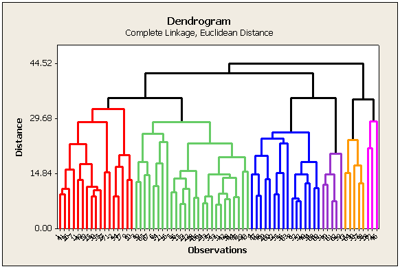
What do you do with the information in this tree diagram?
We decide the optimum number of clusters and which clustering technique to use. We adapted the wood1.sas program to specify the use of the other clustering techniques. Here are links to these program changes. In Minitab also you may select other options instead of a single linkage from the appropriate box.
| File Name | Description of Data |
|---|---|
| wood1.sas | specifies complete linkage |
| wood2.sas | is identical, except that it uses average linkage |
| wood3.sas | uses the centroid method |
| wood4.sas | uses the simple linkage |
As we run each of these programs we must remember to keep in mind that our goal is a good description of the data.
Applying the Cluster Analysis Process
First, we compare the results of the different clustering algorithms. Note that clusters containing one or only a few members are undesirable, as that will give rise to a large number of clusters, defeating the purpose of the whole analysis. That is not to say that we can never have a cluster with a single member! In fact, if that happens, we need to investigate the reason. It may indicate that the single-item cluster is completely different from the other members of the sample and is best left alone.
To arrive at the optimum number of clusters we may follow this simple guideline. Select the number of clusters that have been identified by each method. This is accomplished by finding a breakpoint (distance) below which further branching is ignored. In practice, this is not necessarily straightforward. You will need to try a number of different cut points to see which is more decisive. Here are the results of this type of partitioning using the different clustering algorithm methods on the Woodyard Hammock data. A dendrogram helps determine the breakpoint.
| Cluster Analysis | Linkage Type | Cluster Yield |
|---|---|---|
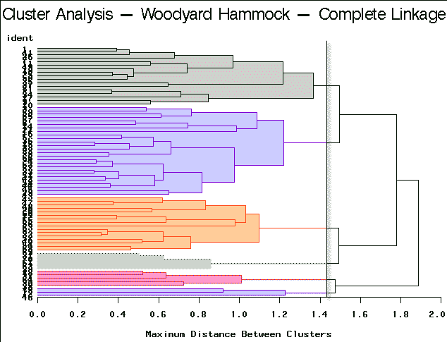 |
Complete Linkage | Partitioning into 6 clusters yields clusters of sizes 3, 5, 5, 16, 17, and 26. |
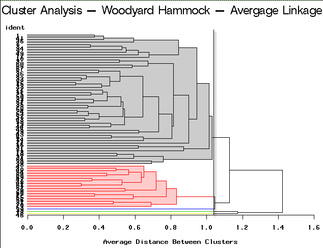 |
Average Linkage | Partitioning into 5 clusters would yield 3 clusters containing only a single site each. |
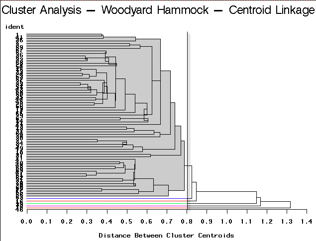 |
Centroid Linkage | Partitioning into 6 clusters would yield 5 clusters containing only a single site each. |
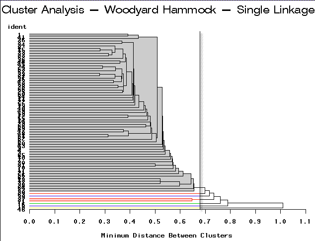 |
Single Linkage | Partitioning into 7 clusters would yield 6 clusters containing only 1-2 sites each. |
For this example, complete linkage yields the most satisfactory result.
For your convenience, the following screenshots demonstrate how alternative clustering procedures may be done in Minitab.